May 16th, SIADS Poster Presentation
This is the online supplement for my poster, my poster at SIADS 2023. Please note that most of content on this site are my personal research notes and are not necessarily intended to be public facing. This page is of course an exception. I will however link to other pages for anyone interested in the details. Consider those pages to be scratchwork that I don't mind sharing.
Traveling Wave Solution
Figure 1 shows some (but not all!) of the variety of traveling wave solutions we see in this model. These solutions are using different parameter values but the same initial conditions, demonstrating that both the parameters and initial conditions determine which traveling wave solution emerges.
For a single set of parameters, we will have either one, or three traveling wave solutions: either a single progressive front (possibly stationary); or a regressive front, a slow unstable progressive front, and a fast stable progressive front.
Pulses have less variety, as "regressive" pulses are simply reflections of progressive pulses. Fronts have asymmetric limiting behaviors so regressive fronts are distinct.
Wave Response
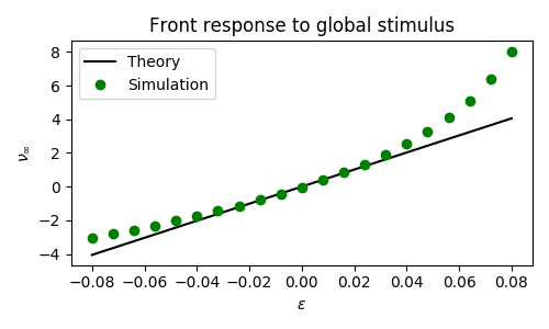
Figure 2 shows how a traveling front responds to a spatially global, instantaneous stimulus. We see that the stimulated pulse eventually stabilizes to a translate of the original front. This translation is called the wave response.
Asymptotics
For details in the asymptotic approximation see Report 2022-05-16. This report is somewhat old and there have since been some small changes to the model. This should give the jist of what the calculations involve.
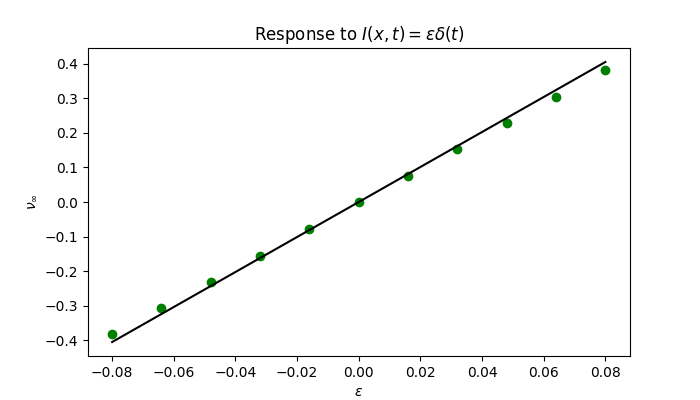
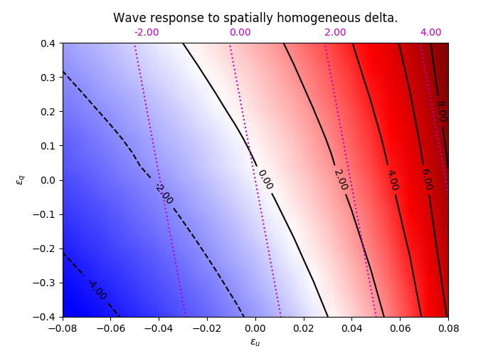
Figures 3, 4, and 5 show front responses to instantaneous global stimuli in both $u$ and $q$. We see that the approximation is quite poor for $q$, even for small stimuli. We believe this is due to the persistence of stimuli in $q$ due to the long time scale, as well as the limitations of the numerical stimulation.
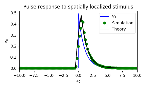
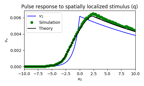
In contrast, when we have local stimulation of pulses, the asymptotic prediction does quite well. Figures 6 and 7 show the effects of small spatially localized stimuli applied to each $u$ and $q$. We see that asymptotic theory matches the simulations and that both predict the wave response will be proportional to the stimulus (narrow square pulse in space) convolved with the null-space of the adjoint.
Details on the derivation of the entrainment condition can be found in report 2023-05-12.