May 16th, 2022
We find the wave response function for the model incorporating synaptic depression. We test our derivation for a spatially homogeneous delta-pulse in the traveling pulse regime.
Wave response
Our neural field model incorporating synaptic depression is given by $$\begin{align*} \mu u_t &= -u + \int_\RR w(x, y) q(y,t) f\big(u(y, t)\big) \ dy + \epsilon I(x, t) \\ \alpha q_t &= 1 - q - \alpha\beta q f(u). \end{align*}$$
In characteristic coordinates $\xi = x - ct$ (and with slight abuse of notation) this becomes $$\begin{align*} -c \mu u_\xi + \mu u_t &= -u + \int_\RR w(\xi, y) q(y,t) f\big(u(y, t)\big) \ dy + \epsilon I(\xi, t) \\ -c \alpha q_\xi + \alpha q_t &= 1 - q - \alpha \beta q f(u). \end{align*}$$
Assume our solution has the expansion $$\begin{align*} u(\xi, t) &= U\big( \xi - \epsilon \nu(t) \big) + \epsilon \phi + \OO(\epsilon^2) \\ q(\xi, t) &= Q\big( \xi - \epsilon \nu(t) \big) + \epsilon \psi + \OO(\epsilon^2) \end{align*}$$ where $U, Q$ denote our traveling pulse solution.
Substituting, and using the linearization $f\big( U + \epsilon \phi + \OO(\epsilon^2) \big) = f(U) + \epsilon f'(U) \phi + \OO(\epsilon^2)$ we have $$\begin{align*} -c\mu (U' + \epsilon \phi_\xi) + \mu (-\epsilon U' \nu' + \epsilon \phi_t) &= -U - \epsilon \phi + \int_\RR w(\xi, y)\big[ Q + \epsilon \psi \big] \big[f(U) + \epsilon f'(U) \phi \big] \ dy + \epsilon I + \OO(\epsilon^2) \\ -c\alpha (Q' + \epsilon \psi_\xi) + \alpha (-\epsilon Q' \nu' + \epsilon \psi_t) &= 1 - Q - \epsilon \psi -\alpha \beta \big(Q + \epsilon \psi\big) \big(f(U) + \epsilon f'(U) \phi \big) + \OO(\epsilon^2) \end{align*}$$ where $U, Q, U'$ and $Q'$ here are understood to be evaluated at $\xi - \epsilon \nu(t)$ (or $y - \epsilon \nu(t)$ when inside the integral).
Collecting the $\OO(1)$ terms, and changing variables $\xi - \epsilon \nu(t) \to \xi$ gives $$\begin{align*} -c\mu U' &= -U + \int_\RR w(\xi, y) Q(y) f(U(y)) \ dy \\ -c\alpha Q' &= 1 - Q - \alpha \beta Q f(U) \end{align*}$$ and is consistent with $U, Q$ being the traveling pulse solution.
Collecting the $\OO(\epsilon)$ terms gives $$\begin{align*} \mu \phi_t + \phi - c\mu \phi_\xi -\int_\RR w(\xi, y) Q(y)f'\big(U(y)\big) \phi(y,t) \ dy - \int_\RR w(\xi, y) f\big(U(y)\big) \psi(y, t) \ dy &= I + \mu U' \nu' \\ \alpha \psi_t + \psi - c\alpha \psi_\xi + \alpha\beta Q f'(U) \phi + \alpha \beta f(U) \psi &= \alpha Q' \nu'. \end{align*}$$ In vector notation this becomes $$\begin{align*} \underbrace{\begin{bmatrix}\mu & 0 \\ 0 & \alpha\end{bmatrix}}_{M} \begin{bmatrix}\phi \\ \psi \end{bmatrix}_t + \underbrace{ \begin{bmatrix}\phi \\ \psi \end{bmatrix} - c\begin{bmatrix}\mu & 0 \\ 0 & \alpha\end{bmatrix} \begin{bmatrix}\phi \\ \psi \end{bmatrix}_\xi + \begin{bmatrix} -w Q f'(U) * \cdot & -w f(U) * \cdot \\ \alpha \beta Q f'(U) & \alpha \beta f(U) \end{bmatrix} \begin{bmatrix}\phi \\ \psi \end{bmatrix} }_{\LL \vecu} &= \begin{bmatrix} I + \mu U' \nu' \\ \alpha Q' \nu ' \end{bmatrix} \end{align*}$$ where $\vecu = [\phi, \psi]^T$ and the convolution operators in the matrix are understood to be applied to the elements of the vector rather than multiplied, in the matrix-vector multiplication.
Bounded solutions exist if the right-hand side is orthogonal to the nullspace of $\LL^*$. We next find this adjoint.
$$\begin{align*} \langle \LL \vecu, \vecv \rangle &= \int \vecv^T \vecu \ d\xi - c\int \vecv^T M \vecu_\xi \ d\xi + \int \vecv^T(\xi) \begin{bmatrix} \int -w(\xi, y) Q(y) f'\big(U(y)\big) \cdot \ dy & \int -w(\xi, y) f\big(U(y)\big) \cdot \ dy \\ \alpha \beta Q f'(U) & \alpha \beta f(U) \end{bmatrix} \vecu \ d\xi \\ &= \int \vecu^T \vecv \ d\xi - c \bigg( \underbrace{\vecv^TM\vecu \bigg|_{\xi = -\infty}^\infty}_{=0} - \int \vecu^T M \vecv_\xi \ d\xi \bigg) + \int \vecu^T(y) \begin{bmatrix} - f'\big(U(y)\big) Q(y) \int w(\xi, y) \cdot d \xi & \alpha \beta Q f'(U) \\ - f(\big(U(y)\big) \int w(\xi, y) \cdot d \xi & \alpha \beta f(U) \end{bmatrix} \vecv \ dy \\ &= \int \vecu^T \vecv \ d\xi + c \int \vecu^T M \vecv_\xi \ d\xi + \int \vecu^T \begin{bmatrix} - f'(U)Q \int w(y, \xi)\cdot d \ y & \alpha \beta Q f'(U) \\ - f(U) \int w(y, \xi) \cdot d y & \alpha \beta f(U) \end{bmatrix} \vecv \ d\xi \\ &= \int \vecu^T \bigg( \underbrace{ \vecv + cM\vecv_\xi + \begin{bmatrix} -f'(U)Q \int w(y, \xi) \cdot \ dy & \alpha \beta Q f'(U) \\ -f(U) \int w(y, \xi) \cdot \ dy & \alpha \beta f(U) \end{bmatrix} \vecv }_{\LL^* \vecv} \bigg) \ d\xi \\ &= \langle \vecu, \LL^* \vecv \rangle \end{align*}$$
Let $[v_1, v_2]^T$ be in the kernel of $\LL^*$. Then they must satisfy $$\begin{align*} -c \mu v_1' &= v_1 -f'(U)Q \int w(y,\xi) v_1(y) \ dy + \alpha \beta Q f'(U)v_2 \\ -c \alpha v_2' &= v_2 - f(U) \int w(y, \xi) v_1(y) \ dy + \alpha \beta f(U) v_2. \end{align*}$$ Our orthogonality condition now becomes $$\begin{align*} 0 &= \int_\RR v_1(I + \mu U' \nu') + v_2(\alpha Q' \nu') \ d\xi \\ &= \nu' \int_\RR \mu U' v_1 + \alpha Q' v_2 \ d\xi + \int_\RR v_1 I \ d\xi \\ \nu'(t) &= - \frac{\int_\RR v_1 I \ d\xi}{\int_\RR \mu U' v_1 + \alpha Q' v_2 \ d\xi} \\ \nu(t) &= - \frac{\int_\RR v_1 \int_0^t I(\xi, \tau) \ d\tau \ d\xi}{\int_\RR \mu U' v_1 + \alpha Q' v_2 \ d\xi}. \end{align*}$$
Our wave response function is given by $$\begin{align*} \nu(t) &= - \frac{\int_\RR v_1 \int_0^t I(\xi, \tau) \ d\tau \ d\xi}{\int_\RR \mu U' v_1 + \alpha Q' v_2 \ d\xi} \end{align*}$$ where $U, Q$ denote the traveling pulse solution, and $v_1, v_2$ satisfy $$\begin{align*} -c \mu v_1' &= v_1 -f'(U)Q \int w(y,\xi) v_1(y) \ dy + \alpha \beta Q f'(U)v_2 \\ -c \alpha v_2' &= v_2 - f(U) \int w(y, \xi) v_1(y) \ dy + \alpha \beta f(U) v_2. \end{align*}$$
Heaviside Firing Rate and bi-exponential weight kernel
Choose $f(\cdot) = H(\cdot - \theta)$ and $w(x,y) = \tfrac{1}{2} e^{-|x - y|}$.We seek $v_1, v_2 \in L^2(\mathbb{R})$ such that $$ \begin{align*} -c \mu v_1' &= v_1 - f'(U)Q \bigg[ \int_{\mathbb{R}} w(y,\xi) v_1(y) \ dy - \alpha \beta v_2\bigg] \\ -c \alpha v_2' &= v_2 - f(U)\bigg[ \int_{\mathbb{R}} w(y, \xi) v_1(y) \ dy - \alpha \beta v_2 \bigg] \end{align*} $$ Rearranging, we have $$ \begin{align*} v_1' + \frac{1}{c\mu} v_1 &= \frac{1}{c\mu}f'(U)Q \bigg[ \int_{\mathbb{R}} w(y,\xi) v_1(y) \ dy - \alpha \beta v_2\bigg] \\ v_2' + \frac{1}{c\alpha}v_2 &= \frac{1}{c\alpha}f(U)\bigg[ \int_{\mathbb{R}} w(y, \xi) v_1(y) \ dy - \alpha \beta v_2 \bigg] \end{align*} $$ Choosing $f(\cdot) = H(\cdot - \theta)$ and $w(x,y) = \tfrac{1}{2} e^{-|x - y|}$ we have $$ \begin{align*} v_1' + \frac{1}{c\mu} v_1 &= \frac{1}{c\mu}\bigg( \frac{\delta(\xi)}{|U'(0)|} + \frac{\delta(\xi + \Delta)}{|U'(-\Delta)|} \bigg)Q \bigg[ \int_{\mathbb{R}} \tfrac{1}{2} e^{-|y - \xi|} v_1(y) \ dy - \alpha \beta v_2\bigg] \\ \big[ e^{\frac{1}{c\mu} \xi} v_1 \big]' &= \frac{1}{c\mu}\bigg( \frac{\delta(\xi)}{|U'(0)|} + \frac{\delta(\xi + \Delta)}{|U'(-\Delta)|} \bigg)Q e^{\frac{1}{c\mu} \xi} \bigg[ \int_{\mathbb{R}} \tfrac{1}{2} e^{-|y - \xi|} v_1(y) \ dy - \alpha \beta v_2\bigg] \\ e^{\frac{1}{c\mu} \xi} v_1 &= A_{-\infty} + \frac{1}{c\mu}\frac{Q(0)}{|U'(0)|} \bigg[ \int_{\mathbb{R}} \tfrac{1}{2}e^{-|y|} v_1(y) \ dy - \alpha \beta v_2(0) \bigg] H(\xi) + \frac{1}{c\mu} e^{-\frac{\Delta}{c\mu}} \frac{Q(-\Delta)}{|U'(-\Delta)|} \bigg[ \int_{\mathbb{R}} \tfrac{1}{2}e^{-|y + \Delta|} v_1(y) \ dy - \alpha \beta v_2(-\Delta) \bigg] H(\xi + \Delta) \\ v_1 &= A_{-\infty}e^{-\frac{1}{c\mu} \xi} + \underbrace{\frac{1}{c\mu}\frac{Q(0)}{|U'(0)|} \bigg[ \int_{\mathbb{R}} \tfrac{1}{2}e^{-|y|} v_1(y) \ dy - \alpha \beta v_2(0) \bigg]}_{A_{0}} e^{-\frac{1}{c\mu} \xi} H(\xi) + \underbrace{\frac{1}{c\mu} e^{-\frac{\Delta}{c\mu}} \frac{Q(-\Delta)}{|U'(-\Delta)|} \bigg[ \int_{\mathbb{R}} \tfrac{1}{2}e^{-|y + \Delta|} v_1(y) \ dy - \alpha \beta v_2(-\Delta) \bigg]}_{A_{-\Delta}} e^{-\frac{1}{c\mu} \xi} H(\xi + \Delta) \\ v_1(\xi) &= A_{-\infty} e^{-\frac{1}{c\mu} \xi} + A_{-\Delta} e^{-\frac{1}{c\mu} \xi} H(\xi + \Delta) + A_{0} e^{-\frac{1}{c\mu} \xi}H(\xi) \end{align*} $$ For $v_1$ to be bounded, we need $0 = \lim\limits_{\xi \to -\infty} v_1(\xi) \implies A_{-\infty} = 0$. This gives two consistency conditions $$ \begin{align*} A_{-\Delta} &= \underbrace{\frac{1}{c\mu} e^{-\frac{\Delta}{c\mu}} \frac{Q(-\Delta)}{|U'(-\Delta)|}}_{D_{-\Delta}} \bigg[ \int \tfrac{1}{2}e^{-|y + \Delta|} \bigg( A_{-\Delta} e^{-\frac{1}{c\mu} y} H(y + \Delta) + A_{0} e^{-\frac{1}{c\mu} y}H(y) \bigg) \ dy - \alpha \beta v_2(-\Delta) \bigg] \\ A_{0} &= \underbrace{\frac{1}{c\mu}\frac{Q(0)}{|U'(0)|}}_{D_0} \bigg[ \int \tfrac{1}{2}e^{-|y|} \bigg( A_{-\Delta} e^{-\frac{1}{c\mu} y} H(y + \Delta) + A_{0} e^{-\frac{1}{c\mu} y}H(y) \bigg) \ dy - \alpha \beta v_2(0) \bigg] \end{align*} $$ or simply \begin{align*} 0 &= \frac{A_{0} D_{-\Delta} \mu c e^{\frac{\Delta}{\mu c}}}{2 \mu c e^{\Delta} e^{\frac{\Delta}{\mu c}} + 2 e^{\Delta} e^{\frac{\Delta}{\mu c}}} + A_{-\Delta} \left(\frac{D_{-\Delta} \mu c e^{\frac{\Delta}{\mu c}}}{2 \mu c + 2} - 1\right) - D_{-\Delta} \alpha \beta \operatorname{v_{2}}{\left(- \Delta \right)} \\ 0 &= A_{0} \left(\frac{D_{0} \mu c}{2 \mu c + 2} - 1\right) + A_{-\Delta} \left(- \frac{D_{0} \mu c e^{\frac{\Delta}{\mu c}}}{2 \mu c e^{\Delta} - 2 e^{\Delta}} + \frac{D_{0} \mu c}{2 \mu c + 2} + \frac{D_{0} \mu c}{2 \mu c - 2}\right) - D_{0} \alpha \beta \operatorname{v_{2}}{\left(0 \right)} \end{align*}
Also, $$\begin{align*} v_2' + \frac{1}{c\alpha}v_2 &= \frac{1}{c\alpha}f(U)\bigg[ \int_{\mathbb{R}} w(y, \xi) v_1(y) \ dy - \alpha \beta v_2 \bigg] \end{align*}$$ and we have $$\begin{align*} v_2' + \frac{1}{c\alpha}v_2 &= 0, &\text{ on } \xi & \not\in (-\Delta, 0) \\ c\alpha v_2' + (1+\alpha\beta)v_2 &= \int_{\mathbb{R}} w(y, \xi) v_1(y) \ dy, & \text{ on } \xi & \in (-\Delta, 0) \end{align*}$$ This integral on the rhs is then $$A_{0} E_{0} e^{\xi} + A_{-\Delta} E_{1} e^{- \xi} + A_{-\Delta} E_{2} e^{- \frac{\xi}{\mu c}}$$ for \begin{align*} E_{0} &= \frac{\mu c}{2 \left(\mu c + 1\right)} \\ E_{1} &= - \frac{\mu c e^{- \Delta + \frac{\Delta}{\mu c}}}{2 \mu c - 2} \\ E_{2} &= \frac{\mu^{2} c^{2}}{\mu^{2} c^{2} - 1}. \end{align*}
Then we have that two outsize pieces are given by $v_2(\xi) \propto e^{-\frac{1}{c\alpha}\xi}$. Since we require $v_2 \in L^2$ the left piece must be zero. The middle piece is given by $$ v_2(\xi) = \frac{A_{0} E_{0} e^{\xi}}{\alpha \beta + \alpha c + 1} - \frac{A_{-\Delta} E_{1} e^{- \xi}}{- \alpha \beta + \alpha c - 1} + \frac{A_{-\Delta} E_{2} \mu e^{- \frac{\xi}{\mu c}}}{\alpha \beta \mu - \alpha + \mu} + C_{1} e^{\frac{\xi \left(- \beta - \frac{1}{\alpha}\right)}{c}} $$ Notice here that we have introduced another unknown variable $C_1$.
Enforcing continuity of $v_2$ gives the final consistency condition $v_2(-\Delta) = 0$. Together these become \begin{align*} 0 &= \frac{A_{0} D_{-\Delta} \mu c e^{\frac{\Delta}{\mu c}}}{2 \mu c e^{\Delta} e^{\frac{\Delta}{\mu c}} + 2 e^{\Delta} e^{\frac{\Delta}{\mu c}}} + A_{-\Delta} \left(\frac{D_{-\Delta} \mu c e^{\frac{\Delta}{\mu c}}}{2 \mu c + 2} - 1\right)\\ 0 &= A_{0} \left(- \frac{D_{0} E_{0} \alpha \beta}{\alpha \beta + \alpha c + 1} + \frac{D_{0} \mu c}{2 \mu c + 2} - 1\right) + A_{-\Delta} \left(\frac{D_{0} E_{1} \alpha \beta}{- \alpha \beta + \alpha c - 1} - \frac{D_{0} E_{2} \alpha \beta \mu}{\alpha \beta \mu - \alpha + \mu} - \frac{D_{0} \mu c e^{\frac{\Delta}{\mu c}}}{2 \mu c e^{\Delta} - 2 e^{\Delta}} + \frac{D_{0} \mu c}{2 \mu c + 2} + \frac{D_{0} \mu c}{2 \mu c - 2}\right) - C_{1} D_{0} \alpha \beta\\ 0 &= \frac{A_{0} E_{0}}{\alpha \beta e^{\Delta} + \alpha c e^{\Delta} + e^{\Delta}} + A_{-\Delta} \left(- \frac{E_{1} e^{\Delta}}{- \alpha \beta + \alpha c - 1} + \frac{E_{2} \mu e^{\frac{\Delta}{\mu c}}}{\alpha \beta \mu - \alpha + \mu}\right) + C_{1} e^{\frac{\Delta}{\alpha c}} e^{\frac{\Delta \beta}{c}} \end{align*} which is linear in $A_{-\Delta}, A_0, C_1$ and amounts to solving a $3 \times 3$ eigenvalue problem.
Our nullspace is given by \begin{align*} v_1(\xi) &= A_{-\Delta} e^{-\frac{1}{c\mu} \xi} H(\xi + \Delta) + A_{0} e^{-\frac{1}{c\mu} \xi}H(\xi) \\ v_2(\xi) &= \begin{cases} 0 & \text{for}\: \Delta < - \xi \\\frac{A_{0} E_{0} e^{\xi}}{\alpha \beta + \alpha c + 1} - \frac{A_{-\Delta} E_{1} e^{- \xi}}{- \alpha \beta + \alpha c - 1} + \frac{A_{-\Delta} E_{2} \mu e^{- \frac{\xi}{\mu c}}}{\alpha \beta \mu - \alpha + \mu} + C_{1} e^{\frac{\xi \left(- \beta - \frac{1}{\alpha}\right)}{c}} & \text{for}\: \xi < 0 \\\left(\frac{A_{0} E_{0}}{\alpha \beta + \alpha c + 1} - \frac{A_{-\Delta} E_{1}}{- \alpha \beta + \alpha c - 1} + \frac{A_{-\Delta} E_{2} \mu}{\alpha \beta \mu - \alpha + \mu} + C_{1}\right) e^{- \frac{\xi}{\mu c}} & \text{otherwise} \end{cases} \end{align*} where $A_{-\Delta}, A_0$ and $C_1$ are non-trivial solutions to the linear system \begin{align*} 0 &= \frac{A_{0} D_{-\Delta} \mu c e^{\frac{\Delta}{\mu c}}}{2 \mu c e^{\Delta} e^{\frac{\Delta}{\mu c}} + 2 e^{\Delta} e^{\frac{\Delta}{\mu c}}} + A_{-\Delta} \left(\frac{D_{-\Delta} \mu c e^{\frac{\Delta}{\mu c}}}{2 \mu c + 2} - 1\right)\\ 0 &= A_{0} \left(- \frac{D_{0} E_{0} \alpha \beta}{\alpha \beta + \alpha c + 1} + \frac{D_{0} \mu c}{2 \mu c + 2} - 1\right) + A_{-\Delta} \left(\frac{D_{0} E_{1} \alpha \beta}{- \alpha \beta + \alpha c - 1} - \frac{D_{0} E_{2} \alpha \beta \mu}{\alpha \beta \mu - \alpha + \mu} - \frac{D_{0} \mu c e^{\frac{\Delta}{\mu c}}}{2 \mu c e^{\Delta} - 2 e^{\Delta}} + \frac{D_{0} \mu c}{2 \mu c + 2} + \frac{D_{0} \mu c}{2 \mu c - 2}\right) - C_{1} D_{0} \alpha \beta\\ 0 &= \frac{A_{0} E_{0}}{\alpha \beta e^{\Delta} + \alpha c e^{\Delta} + e^{\Delta}} + A_{-\Delta} \left(- \frac{E_{1} e^{\Delta}}{- \alpha \beta + \alpha c - 1} + \frac{E_{2} \mu e^{\frac{\Delta}{\mu c}}}{\alpha \beta \mu - \alpha + \mu}\right) + C_{1} e^{\frac{\Delta}{\alpha c}} e^{\frac{\Delta \beta}{c}} \end{align*} with \begin{align*} E_{0} &= \frac{\mu c}{2 \left(\mu c + 1\right)} \\ E_{1} &= - \frac{\mu c e^{- \Delta + \frac{\Delta}{\mu c}}}{2 \mu c - 2} \\ E_{2} &= \frac{\mu^{2} c^{2}}{\mu^{2} c^{2} - 1} \\ D_{-\Delta} &= \frac{1}{c\mu} e^{-\frac{\Delta}{c\mu}} \frac{Q(-\Delta)}{|U'(-\Delta)|} \\ D_{0} &= \frac{1}{c\mu} \frac{Q(0)}{|U'(0)|} \end{align*}
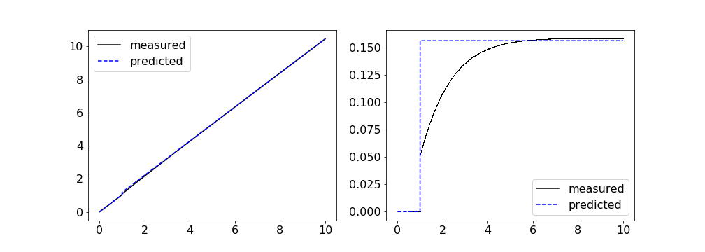
Below is a simulation showing a traveling pulse with parameters \begin{align*} \theta &= 0.2\\ \alpha &= 20\\ \beta &= 0.25\\ \mu &= 1 \end{align*} responding to the stimulus $\epsilon I(x,t) = \epsilon \delta(t - 1)$. The animation and Figure 1 show the response and our asymptotic approximation for $\epsilon = 0.1$. Figure 2 shows the response and our approximation for $\epsilon = 0.01$. We see that the asymptotic approximation converges to the simulated response as $\epsilon \to 0$.