May 12th, 2023
Zack had a clever idea for the asymptotic expansion. This new expansion allows us to get a differential equation for the wave response which can successfully predict entrainment for weak stimuli. We walk through the derivation in the scalar case (no synaptic depression) for a moving Heaviside stimulus. For the pulse regime in the synaptic depression model we also consider a moving Heaviside, and a moving square wave.
Asymptotic Entrainment Calculation
We consider the scalar equation $$ u_t = -u + w \ast f[u]. $$ In characteristic coordinates (and with a slight abuse of notation) this is $$ -cu_\xi + u_t = -u + w\ast f[u]. $$
For a small stimulus term $\varepsilon I(\xi, t)$ we use the expansion $$\begin{align*} u(\xi, t) &= U(\xi - \varepsilon \nu(t)) + \varepsilon \phi(\xi - \varepsilon \nu, t) + \mathcal{O}(\varepsilon^2) \\ u_\xi &= U' + \varepsilon \phi_\xi + \mathcal{O}(\varepsilon^2) \\ u_t &= -\varepsilon \nu' U' -\varepsilon^2 \nu' \phi_\xi + \varepsilon \phi_t + \mathcal{O}(\varepsilon^2) \\ &= -\varepsilon \nu' U' + \varepsilon \phi_t + \mathcal{O}(\varepsilon^2) \end{align*}$$
Substituting, and collecting the $\mathcal{O}(\varepsilon)$ terms, we have $$\begin{align*} -c\phi_\xi - \nu'U' + \phi_t &= -\phi + w \ast \big(f'[U]\phi \big) I(\xi + \varepsilon \nu, t) \\ \phi_t + \underbrace{\phi - c\phi_\xi - w \ast \big( f'[U] \phi \big)}_{\mathcal{L}} &= \nu'U' + I(\xi + \varepsilon \nu, t). \end{align*}$$
We require the RHS to be orthogonal to every term in the nullspace of $\mathcal{L}^*$. This one-dimensional null-space is spanned by $v(\xi) = H(\xi)e^{-\xi / c}$. This gives our wave response as $$ \nu' = -\frac{ \langle I(\xi + \varepsilon \nu, t), v \rangle}{\langle U', v \rangle}. $$
From Kilpatrick 2012 we have $U'(\xi) = -\frac{1}{2(c+1)}e^{-\xi}$. Thus $$\begin{align*} \langle U', v \rangle &= -\frac{1}{2(c+1)}\int_0^\infty e^{-\xi} e^{-\xi/c} d \xi \\ &= -\int_0^\infty e^{- \frac{1+c}{c} \xi} \ d\xi \\ &= -\frac{c}{2(c+1)^2}. \end{align*}$$
We will take $\varepsilon I$ to be a moving Heaviside stimulus $$ \varepsilon I(\xi, t) = \varepsilon H\big( -(\xi - \Delta_c t) \big). $$ Thus $$\begin{align*} \langle I(\xi + \varepsilon \nu), v \rangle &= \int_0^\infty e^{-\xi / c} H\big( -( \xi + \varepsilon \nu - \Delta_c t) \big) d \xi \\ &= \int_0^{\Delta_c t - \varepsilon \nu} e^{-\xi/c} \ d\xi \\ &= c (1 - e^{\frac{\varepsilon \nu - \Delta_c t}{c}}) \end{align*}$$ and our wave response satisfies $$ \nu' = 2(c+1)^2(1 - e^{\frac{\varepsilon \nu - \Delta_c t}{c}}). $$
We make the change of variables $$\begin{align*} y(t) &= \frac{ \varepsilon \nu - \Delta_c t}{c} \\ \nu &= \frac{y + \Delta_c t}{\varepsilon} \\ \nu' &= \frac{y' + \Delta_c}{\varepsilon} \end{align*}$$ and substitute to obtain $$\begin{align*} \frac{y' + \Delta_c}{\varepsilon} &= 2(c+1)^2(1 - e^y) \\ y' &= -\Delta_c + 2 \varepsilon(c+1)^2(1 - e^y) := F(y). \end{align*}$$
A traveling wave solution will reach a steady state where $\nu'(t) = \Delta_c$ or equivalently $y' = 0$. Such a steady state $\bar{y}$ satisfies $$\begin{align*} 0 &= F(\bar{y}) \\ &= -\Delta_c + 2 \varepsilon(c+1)^2(1 - e^\bar{y}) \\ \frac{\Delta_c}{2\varepsilon(c+1)^2)} &= 1 - e^{\bar{y}} \\ \bar{y} &= \log \left( 1 - \frac{\Delta_c}{2\varepsilon(c+1)^2)} \right). \end{align*}$$
This will be stable if $F'(\bar{y}) < 0$. We check $$\begin{align*} F'(\bar{y}) &= -2\varepsilon (c+1)^2 e^\bar{y} \\ &= -2\varepsilon (c+1)^2 \left( 1 - \frac{\Delta_c}{2\varepsilon (c+1)^2} \right) \\ &= \Delta_c - 2\varepsilon(c+1)^2. \end{align*}$$ This will be negative if $$ \Delta_c < 2\varepsilon(c+1)^2. $$
Comparison to constant input
Suppose that the stimulus is too fast. Then we have essentially that $\varepsilon I \to \varepsilon$ as $t \to \infty$. As the stimulus moves farther ahead of the front, the front will accelerate until it reaches some maximum speed. This maximum speed must be less than the speed of the stimulus otherwise the speeds would eventually match and the front would entrain to the stimulus. This gives a condition on the stimulus speed.
In the case of the stimulus $\varepsilon I = \varepsilon$ we make the change of variables $\hat{u} = u - \varepsilon$ $\hat{\theta} = \theta - \varepsilon$ and we obtain the original unperturbed equation in $\hat{u}$. Thus, we expect $$\begin{align*} \hat{c} = c + \Delta_c &= \frac{1}{2\hat{\theta}} - 1 \\ \Delta_c &= \frac{1}{2(\frac{1}{2(c+1)} - \varepsilon)} - 1 - c \\ &= \frac{c+1}{1 - 2(c+1)\varepsilon} - (1+c) \\ &= 2\varepsilon(c+1)^2 + \mathcal{O}(\varepsilon^2) \end{align*}$$ which is consistent with the above analysis to first order.
Synaptic Depression with moving Heaviside stimulus
The model incorporating synaptic depression similarly yields the wave response equation $$ \nu' = \frac{ \langle v_1, I_u(\xi + \varepsilon \nu) \rangle + \langle v_2, I_q(\xi + \varepsilon \nu) \rangle }{ \underbrace{-\tau_u \langle v_1, U' \rangle - \tau_q \langle v_2, Q' \rangle}_{D} }. $$ We will take the stimulus $\varepsilon I_q = 0$ and $\varepsilon I_u(\xi, t) = H(-(\xi - \Delta_c t))$ and the relevant nullspace equation is $$ v_1(\xi) = A_{-\Delta} H(\xi + \Delta) e^{-\xi/c\tau_u} + H(\xi)e^{-\xi/c\tau_u}. $$
We then have $$\begin{align*} D \nu' &= \langle v_1, I_u(\xi + \varepsilon \nu) \rangle \\ &= \int_0^\infty H(-(\xi + \varepsilon \nu - \Delta_c t))e^{-\xi/c\tau_u} \ d\xi + \int_{-\Delta}^\infty H(-(\xi + \varepsilon \nu - \Delta_c t)) e^{-\xi/c\tau_u} \ d\xi \\ &= \int_0^{\Delta_c t - \varepsilon \nu} e^{-\xi/c\tau_u} \ d\xi + A_{-\Delta} \int_{-\Delta}^{\Delta_c t - \varepsilon \nu} e^{-\xi/c\tau_u} \ d\xi \\ &= c\tau_u \bigg( (1 - e^{\frac{\varepsilon \nu - \Delta_c t}{c \tau_u}}) + A_{-\Delta}(e^{\Delta/c\tau_u} - e^{\frac{\varepsilon \nu - \Delta_c t}{c \tau_u}}) \bigg) \\ &= c\tau_u (1 + A_{-\Delta}e^{\Delta/c\tau_u}) - c\tau_u(1+A_{-\Delta})e^{\frac{\varepsilon \nu - \Delta_c t}{c \tau_u}}. \end{align*}$$
Similarly to before, we make the change of variables $y(t) = \varepsilon \nu(t) - \Delta_c t$. If $\varepsilon \nu(t)$ is the location of the fore threshold crossing in the traveling wave coordinate frame, $y(t)$ is the location of the fore threshold crossing in the stimulus coordinate frame (speed $c + \Delta_c$). This gives $$\begin{align*} D \frac{y' + \Delta_c}{\varepsilon} &= c\tau_u (1 + A_{-\Delta}e^{\Delta/c\tau_u}) - c\tau_u(1+A_{-\Delta})e^{y/c\tau_u} \\ y' &= -\Delta_c + \frac{\varepsilon c \tau_u}{D} \bigg( (1 + A_{-\Delta}e^{\Delta/c\tau_u}) - (1+A_{-\Delta})e^{y/c\tau_u} \bigg) := F(y). \end{align*}$$
This has a steady state at $$\begin{align*} 0 &= F(\bar{y}) \\ &= -\Delta_c + \frac{\varepsilon c \tau_u}{D} \bigg( (1 + A_{-\Delta}e^{\Delta/c\tau_u}) - (1+A_{-\Delta})e^{\bar{y}/c\tau_u} \bigg) \\ e^{\bar{y}/c\tau_u} &= \frac{-\frac{D \Delta_c}{\varepsilon c \tau_u} + (1 + A_{-\Delta}e^{\Delta/c\tau_u}) }{ 1 + A_{-\Delta}} \tag{*} \\ \bar{y} &= c\tau_u \log \left( \frac{(1 + A_{-\Delta}e^{\Delta/c\tau_u}) -\frac{D \Delta_c}{\varepsilon c \tau_u}}{ 1 + A_{-\Delta}} \right). \end{align*}$$ This steady state is stable if $$\begin{align*} 0 &> F'(\bar{y}) \\ &= - \frac{\varepsilon (1 + A_{-\Delta})}{D} e^{\bar{y} /c\tau_u} \tag{substitute (*)} \\ &= - \frac{\varepsilon (1 + A_{-\Delta})}{D} \frac{-\frac{D \Delta_c}{\varepsilon c \tau_u} + (1 + A_{-\Delta}e^{\Delta/c\tau_u}) }{ 1 + A_{-\Delta}} \\ &= \frac{\Delta_c}{c \tau_u} - \frac{\varepsilon}{D}(1 + A_{-\Delta}e^{\Delta/c\tau_u}) \\ \Delta_c &< \varepsilon \frac{c\tau_u}{D}(1+A_{-\Delta}e^{\Delta/c\tau_u}). \end{align*}$$
A note on a moving square stimulus
In the $\tau_q \gg \tau_u$ regime, we expect $A_{-\Delta} \approx 0$. In this case, there are no effects from the rear threshold-crossing. Then if we consider a moving square stimulus of width $y^*$ $$ \varepsilon I_u(\xi, t) = \varepsilon \bigg( H( - (\xi - \Delta_c t)) - H(\xi - \Delta_c t y^*) \bigg) $$ then our analysis will be identical to the above provided $-\bar{y} > y^*$. That is, if the back end of the square stimulus is in the active region of the steady-state perturbed traveling wave. I suspect that this will be a requisite condition on entrainment for the square stimulus case.
Specifically, the effect of the stimulus on an entrained traveling wave would be maximal when the rear end of the stimulus is at the threshold crossing. If this effect from the stimulus is too strong, then the wave will advance and the rear of the stimulus will be in the active region. If this effect from the stimulus is too weak, then the wave would lag behind and the effect from the stimulus will lessen even more.
In this regime the comparison to a constant stimulus will similarly be relevant, though the speed (and pulse width) is specified implicity. Still, it may be possible to derive a first order approximation to the entrainment condition.
Moving square stimulus
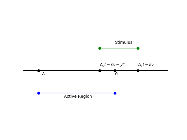
We next consider a moving square stimulus of the form $$ \varepsilon I_u(\xi, t) = \varepsilon \bigg[ H\big( -(\xi - \Delta_c t) \big) - H\big(-(\xi + y^* - \Delta_c t) \big) \bigg] $$ where $y^*$ is the width of the stimulus and $\Delta_c$ is the speed of the stimulus in the unperturbed traveling wave coordinate frame. Our entrainment calculation now has several cases. In the $\tau_q \gg \tau_u$ parameter regime, we expect the pulse width to be large, so we will assume $y^* \ll \Delta$. Also, the effect from the rear of the pulse is vanishingly small so we expect the front of the stimulus to be ahead of the fore threshold crossing. This reduces us to two cases: one where the back of the stimulus is in the active region and one where the back of the stimulus is ahead of the pulse. Intuitively we expect that if the rear of the stimulus is ahead of the pulse this will have a weaker effect than if the rear of the stimulus were at $\xi = 0$, and thus such a solution will be unstable. Therefore we choose to first consider the case where the stimulus overlaps with the active region, as seen in the diagram below.
Our wave response is then give by $$\begin{align*} \underbrace{ \tau_u \langle v_1, U' \rangle }_{D} \nu' &= \langle v_1, I(\xi + \varepsilon \nu, t) \rangle \\ &= \int_0^{\Delta_c t - \varepsilon \nu} e^{-\xi/c\tau_u} \ d\xi + A_{-\Delta} \int_{\Delta_c t - \varepsilon \nu - y^*}^{\Delta_c t - \varepsilon \nu} e^{-\xi/c\tau_u} \ d\xi \\ &= c\tau_u \left[1 - \exp\left(\frac{\varepsilon \nu - \Delta_c t}{c \tau_u}\right)\right] + c\tau_u A_{-\Delta} \left[ \exp\left(\frac{y^* + \varepsilon \nu - \Delta_c t}{c \tau_u}\right) - \exp\left(\frac{\varepsilon \nu - \Delta_c t}{c \tau_u}\right) \right] \\ &= c \tau_u \left[ 1 + \left( A_{-\Delta} e^{y^*/c\tau_u} -(1+A_{-\Delta}) \right) \exp\left(\frac{\varepsilon \nu - \Delta_c t}{c \tau_u}\right) \right] \\ \nu' &= \frac{c \tau_u}{D} \left[ 1 + \left( A_{-\Delta} e^{y^*/c\tau_u} -(1+A_{-\Delta}) \right) \exp\left(\frac{\varepsilon \nu - \Delta_c t}{c \tau_u}\right) \right]. \end{align*}$$
Define $y = \varepsilon \nu - \Delta_c t$ to be the distance between the fore threshold crossing and the front of the stimulus. Then $\nu' = \frac{y' + \Delta_c}{\varepsilon}$ and $$\begin{align*} \frac{y' + \Delta_c}{\varepsilon} &= \frac{c \tau_u}{D} \left[ 1 + \left( A_{-\Delta} e^{y^*/c\tau_u} -(1+A_{-\Delta}) \right) e^{y/c\tau_u} \right] \\ y' &= -\Delta_c + \frac{ \varepsilon c \tau_u}{D} \left[ 1 + \left( A_{-\Delta} e^{y^*/c\tau_u} -(1+A_{-\Delta}) \right) e^{y/c\tau_u} \right] := F(y). \end{align*}$$
This has a steady state $\bar{y}$ give by $$\begin{align*} 0 &= F(\bar{y}) \\ &= -\Delta_c + \frac{ \varepsilon c \tau_u}{D} \left[ 1 + \left( A_{-\Delta} e^{y^*/c\tau_u} -(1+A_{-\Delta}) \right) e^{\bar{y}/c\tau_u} \right] \\ \frac{\Delta_c D}{\varepsilon c \tau_u} &= 1 + \left( A_{-\Delta} e^{y^*/c\tau_u} -(1+A_{-\Delta}) \right) e^{\bar{y}/c\tau_u} \\ e^{\bar{y}/c\tau_u} &= \frac{1 - \frac{\Delta_c D}{\varepsilon c \tau_u}}{1 + A_{-\Delta} - A_{-\Delta}e^{y^*/c\tau_u}} \\ \bar{y} &= c\tau_u \log\left( \frac{1 - \frac{\Delta_c D}{\varepsilon c \tau_u}}{1 + A_{-\Delta} - A_{-\Delta}e^{y^*/c\tau_u}} \right). \end{align*}$$ Note that we require $0 > \bar{y} - y^* > \Delta$ in order for the rear of the stimulus to be in the active region, which is consistent with this case.
We have stability if $$\begin{align*} 0 &> F'(\bar{y}) \\ &= \frac{\varepsilon }{D} \left( A_{-\Delta} e^{y^*/c\tau_u} -(1+A_{-\Delta}) \right) e^{\bar{y}/c\tau_u} \\ &= \frac{\varepsilon }{D} \left( A_{-\Delta} e^{y^*/c\tau_u} -(1+A_{-\Delta}) \right) \frac{1 - \frac{\Delta_c D}{\varepsilon c \tau_u}}{1 + A_{-\Delta} - A_{-\Delta}e^{y^*/c\tau_u}} \\ &= \frac{\varepsilon}{D} \left( \frac{\Delta_c D}{\varepsilon c\tau_u} - 1 \right) \\ &= \frac{\Delta_c}{c \tau_u} - \frac{\varepsilon}{D} \\ \Delta_c &< \frac{\varepsilon c \tau_u}{D}. \end{align*}$$
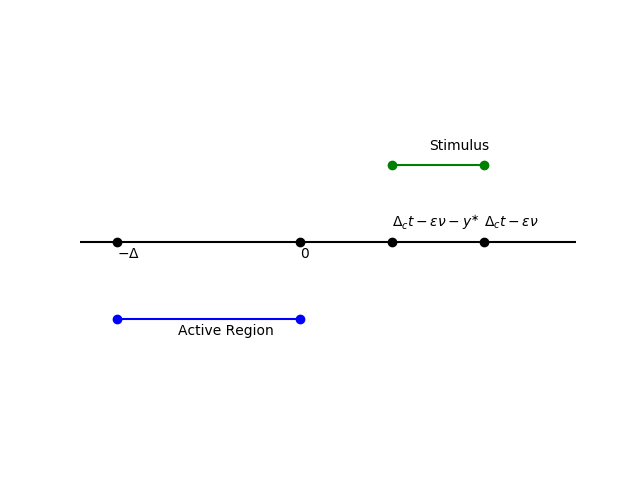
The inconsistent case
We postulated that the case where the rear of the stimulus is ahead of the pulse is inconsistent. Here, we justify that analytically. This case is depicted in the following diagram.
We proceed $$\begin{align*} D\nu' &= \int_{\Delta_c t - \varepsilon \nu - y^*}^{\Delta_c t - \varepsilon \nu} e^{-\xi/c\tau_u} \ d\xi + A_{-\Delta} \int_{\Delta_c t - \varepsilon \nu - y^*}^{\Delta_c t - \varepsilon \nu} e^{-\xi/c\tau_u} \ d\xi \\ &= c\tau_u(1+A_{-\Delta}) \left[ \exp\left(\frac{y^* + \varepsilon \nu - \Delta_c t}{c\tau_u} \right) - \exp\left(\frac{\varepsilon \nu - \Delta_c t}{c\tau_u} \right) \right] \\ &= c\tau_u(1+A_{-\Delta}) \exp\left(\frac{\varepsilon \nu - \Delta_c t}{c \tau_u} \right) \left( e^{y^*/c\tau_u} - 1 \right). \end{align*}$$
We change variables $y = \varepsilon \nu - \Delta_c t$ and $\nu' = \frac{y' + \Delta_c}{\varepsilon}$ yielding $$\begin{align*} \frac{D}{\varepsilon} (y' + \Delta_c) &= c\tau_u(1+A_{-\Delta}) e^{y/ c \tau_u} \left( e^{y^*/c\tau_u} - 1 \right) \\ y' &= -\Delta_c + \frac{\varepsilon c \tau_u (1+A_{-\Delta})}{D} \left( e^{y^*/c\tau_u} - 1 \right) e^{y/ c \tau_u} := F(y). \end{align*}$$
We have a steady state at $$\begin{align*} 0 &= F(\bar{y}) \\ &= -\Delta_c + \frac{\varepsilon c \tau_u (1+A_{-\Delta})}{D} \left( e^{y^*/c\tau_u} - 1 \right) e^{\bar{y}/ c \tau_u} \\ e^{\bar{y}/c\tau_u} &= \frac{\Delta_c D}{\varepsilon c\tau_u (1+A_{-\Delta}) \left( e^{y^*/c\tau_u} - 1 \right) } \\ \bar{y} &= c\tau_u \log \left( \frac{\Delta_c D}{\varepsilon c\tau_u (1+A_{-\Delta}) \left( e^{y^*/c\tau_u} - 1 \right) } \right). \end{align*}$$
However, this solution is unstable as shown by the following calculation $$\begin{align*} 0 &> F'(\bar{y}) \\ &= \frac{\varepsilon (1+A_{-\Delta})}{D}(e^{y^*/c\tau_u} - 1) e^{\bar{y}/c\tau_u} \\ &= \frac{\varepsilon (1+A_{-\Delta})}{D}(e^{y^*/c\tau_u} - 1) \frac{\Delta_c D}{\varepsilon c\tau_u (1+A_{-\Delta}) \left( e^{y^*/c\tau_u} - 1 \right) } \\ &= \frac{\Delta_c}{c\tau_u} \end{align*}$$ which is a contradiction since all terms are positive.
Final Comments
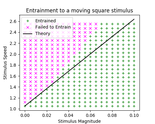
I've compared this approximation to simulations in the case of a moving square wave perturbing a traveling pulse. As seen below, this is a good approximation to the domain of entrainment for small $\varepsilon$.
 For the paper, I think it would be better to instead use the substitution
$$
y(t) = \Delta_c t - \varepsilon \nu(t).
$$
Then $\bar{y}$ would be positive and would be the distance from the active region to the front of the stimulus. The condition that $\bar{y}$ is less than the stimulus width ($y^*$) will give a stronger condition. In effect, it multiplies the slope by roughly $1 - e^{y^*/c\mu}$. For wide stimuli this factor is roughly 1. This is consistent with the figure above. It will be good to also test this approximation for thin stimuli.
For the paper, I think it would be better to instead use the substitution
$$
y(t) = \Delta_c t - \varepsilon \nu(t).
$$
Then $\bar{y}$ would be positive and would be the distance from the active region to the front of the stimulus. The condition that $\bar{y}$ is less than the stimulus width ($y^*$) will give a stronger condition. In effect, it multiplies the slope by roughly $1 - e^{y^*/c\mu}$. For wide stimuli this factor is roughly 1. This is consistent with the figure above. It will be good to also test this approximation for thin stimuli.