June 17th, 2021
We numerically verify the wave response calculated in the previous report and motivate the need for a higher order method.
To-Do List Snapshot
- Investigate wave-response function.
Spatially homogeneous pulse.- Spatially homogeneous, temporally finite.
- Local pulses.
- Wave-train Analysis
- Search the literature.
- Find periodic solutions.
- Compare frequency to a pair of pulses.
- Reading
- Coombes 2004.
- Folias & Bressloff 2005.
- Faye & Kilpatrick 2018.
Some Corrections
Figure 3 in report 2021-06-03 was incorrectly interpreted as ill-conditioned in the computation of the pulse-speed. The calculation of the pulse-speed $c \approx 4$ is very well-conditioned as the derivative is large near the root. However, the formula for the pulse-width is very sensitive to the value of $c$ as $c \to 4$ making numerical approximation of the pulse-width, and by extension the traveling pulse soltuion, infeasible.
There was a small error in the previous report in the calculation of the asymptotic approximation of the wave repsonse function for the specific example chosen. The correct formula is used below.
Spatially Homogeneous Pulse Stimulus
Last week (report 2021-06-10) we have derived the wave-response function $$ \epsilon \nu(t) = \frac{\mu c+1}{\mu^2 c \theta} \int_0^t \int_0^\infty e^{-\xi/c\mu} \epsilon I(\xi, t) \ d\xi \ d\tau $$ for general stimului $\epsilon I(\xi, t)$. We further simplified this for the case $\epsilon I(\xi, t) = I_0 \delta(t - t_0)$ to obtain $$ \nu(t) = \frac{\mu c+1}{\mu \theta} I_0. $$
The rest of the report focused on certain numerical difficulties in measuring the pulse-speed and pulse-width when simulating an unperturbed traveling pulse solution, in anticipation of these difficulties confounding our attempts to numerically verify our asymptotic approximation of the wave-response function. Such a discussion is more clearly motivated by first attempting said verification.
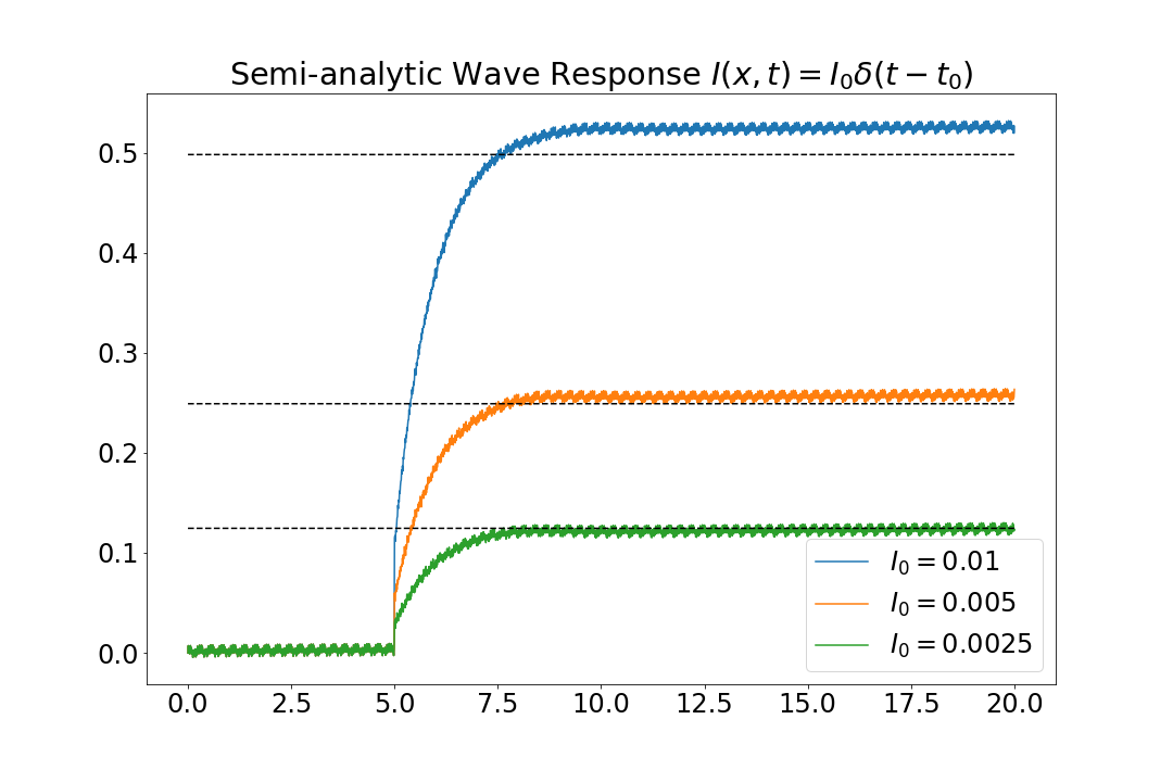
In Figure 1, we attempt to create a plot similar to Figure 3(b) in Kilpatrick & Bressloff 2010, comparing the measured wave response from a stimulus $I(x, t) = I_0 \delta(t - t_0)$ to our asymptotic approximation. Initially, the results are promising, but this is slightly deceptive. Figure 1 does not use the value $c_\text{analytic} = 3.9999$ found by root-finding as specified in report 2021-06-03. We will refer to this as the analytic value, as it is the numerical result from a well-conditioned analytic formula. Figure 1 does not use this analytic value, but rather it simulates the traveling wave solution, measures the pulse-speed before stimulation, and uses this measured value for $c_\text{measured} \approx 3.9802$ in the asymptotic formula. We will call this the measured value.
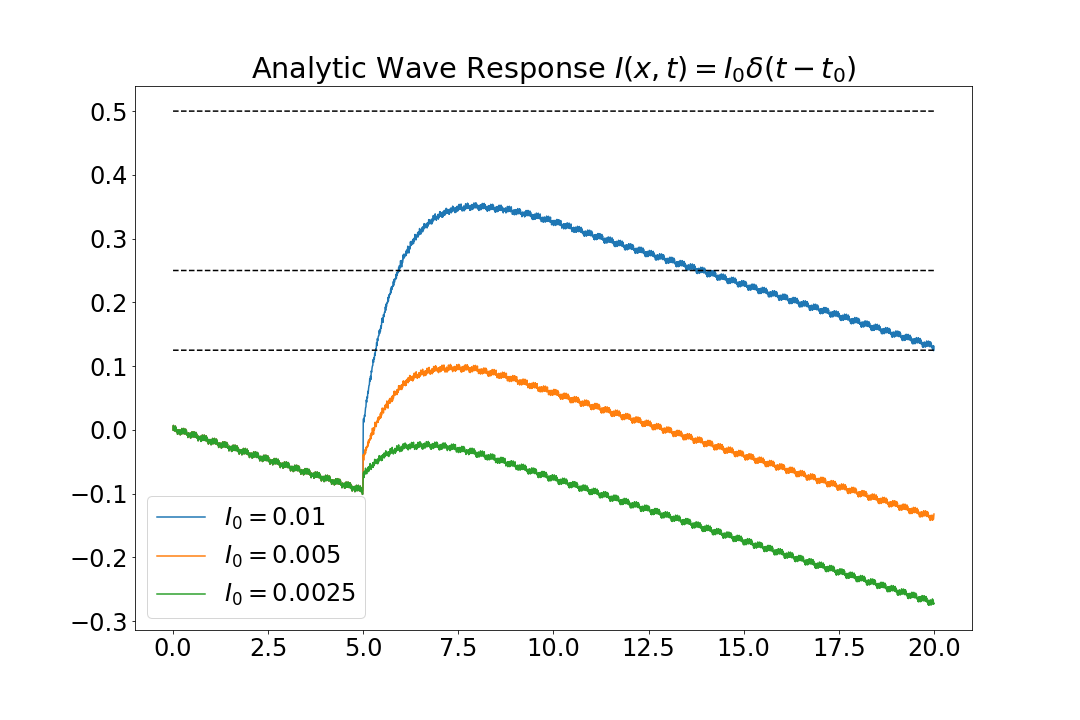
Lastly, Figure 3 shows measured wave response function, adjusted for the measured speed, compared to the asymptotic approximation using the analytically computed speed. This is, perhaps, a more honest comparison. The difference in Figures 1 and 3 is only in asymptotic approximation.

As the asymptotic approximation is affine in $c$, the constant difference is given by $$ \nu_\text{analytic}(t) - \nu_\text{measured}(t) = (c_\text{analytic} - c_\text{measured}) \frac{I_0}{\theta}. $$ Visually the difference is still small, but but a more precise comparison in the form of a convergence study would put any uncertainty to rest. This has proven difficult, as the front locations, relative to the pulse-speed, do not converge to a constant value, but rather ocillate rappidly between time-steps.
Simulation Convergence
The measurment errors and ocillations are presumably due to the large grid-spacing in the spatial dimension and the low-order accuracy of the convolution. The convergence study in Figures 4 and 5 would seem to confirm this. They show our measurements of the speed and width over the course of a simulation for a series of simulations with progressivly smaller grid-spacing. These simulations do not incorporate external sitmuli and are initialized with our analytic formula for the traveling wave soltuion.
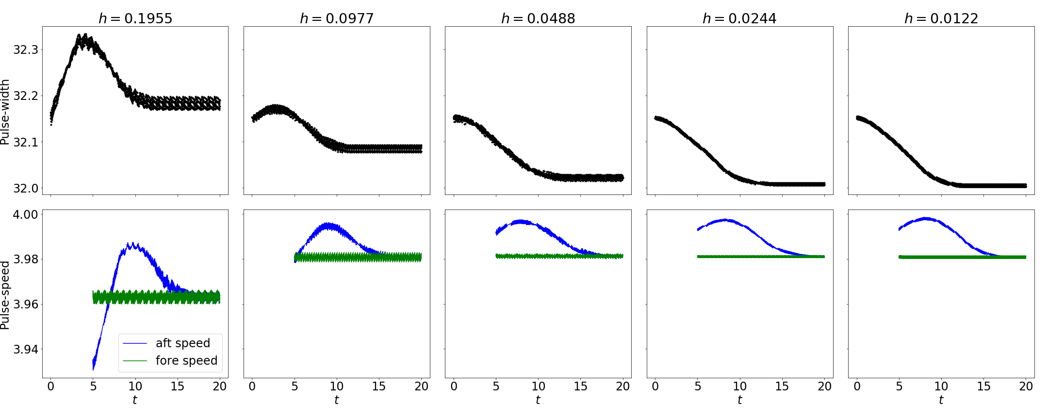
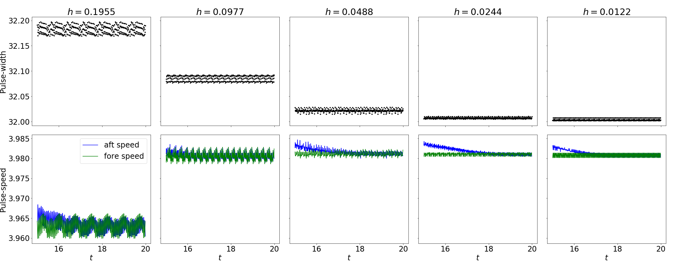
We see that the solutions seem to be converging (though not to our predicted speed and pulse-width) up to a point, but the oscilations remain. We expect that a higher order algorithm will give better results
Improving Accuracy
Presently, the accuracy and speed of our simulations is limited by the convolution step. We precompute a dense matrix for the weight function and then perform the convolution by applying this matrix to the output of the firing-rate function. The matrix multiplication limits our speed as it has $O(n^2)$ complexity, and the discretization of the non-smooth Heaviside firing-rate function limits our accuracy to $O(h)$ (despite using the trapezoidal rule).
We can improve this by calculating the convolution semi-analytically, using the treshold-crossing locations as we have for previous models. However, in this case, locating these locations to higher than $O(h)$ is more difficult due to the non-smoothness of the solutions. Using polynomial interpolation to find the threshold-crossings more accurately fails since it requires smoothness of the underlying function.
We propose the following work-around that should identify the threshold-crossings to higher order:
- Locate the threshold-crossings to first order, by identifying the two grid points on either side, which will will call the bounding grid points.
- Apply a three-point second-derivative finite difference stencil to nearby grid ponits to identify cusps (jumps in the first derivative).
- Use the cusp locations to select between the following interpolation shchemes:
- If a cusp does not occur near our threshold-crossing, improve the approximation by interpolating nearby grid points
- If a cusp occurs near our threshold-crossing, but not between the bounding grid points, use a one-sided polynomial interpolation over points that do not include the cusp.
- If a cusp occurs between the bounding grid points, find separate polynomial interpolants for each side, locate their intersection point, and use the intersection point to determine which polynomial will be used to approximate the threshold-crossing.