June 3rd, 2021
We finished deriving the traveling pulse solution. We encountered a bug in SymPy's integration routine involving the Heaviside function and variable assumptions, which cause delays. We submitted a bug report and proceeded integrating the forcing term by hand. The choice of parameters for our simulation makes determining the pulse width and wave speed an ill-conditioned process. We began simulations for spatially homogeneous temporally pulsatile stimuli.
To-Do List Snapshot
Analytically find the traveling pulse/front solutions.- Investigate wave-response function.
- Spatially homogeneous pulse.
- Spatially homogeneous, temporally finite.
- Local pulses.
- Wave-train Analysis
- Search the literature.
- Find periodic solutions.
- Compare frequency to a pair of pulses.
- Reading
- Coombes 2004.
- Folias & Bressloff 2005.
- Faye & Kilpatrick 2018.
Traveling Pulses
The non-linear adaptation model is the model from Kilpatrick & Bressloff 2010 (KB10) but with the synaptic depression ($q$) removed. This is equivalent to setting $\beta = 0$ and initializing $q = 1$ in their model. The result is then $$\begin{align*} \mu u_t &= -u + \int_{-\infty}^\infty w(x,x^\prime) f( u(x^\prime,t) - a(x^\prime,t)) \ dx^\prime \\ \alpha a_t &= -a + \gamma f(u - a). \end{align*}$$ Note that we have re-labeled the parameters $\epsilon \to \alpha$ and the old $\alpha$ is not present.
Assume a Heaviside firing rate function, the exponential weight function $$\begin{align*} f(u-a) &= H(u-a - \theta) \\ w(x, x^\prime) &= \tfrac{1}{2} e^{-|x-x^\prime|}. \end{align*}$$
Ultimately this gives the traveling pulse solution $$\begin{align*} u(x,t) = U{\left(\xi \right)} &= \begin{cases} \frac{\left(- \frac{e^{\Delta}}{\mu c - 1} + \frac{1}{\mu c - 1}\right) e^{\xi}}{2} + \frac{\left(\mu^{2} c^{2} e^{\frac{\Delta}{\mu c}} - \mu^{2} c^{2} - \frac{\mu c}{2} + \theta \left(\mu^{2} c^{2} - 1\right) + \frac{\left(\mu c - 1\right) e^{- \Delta}}{2} + \frac{1}{2}\right) e^{\frac{\xi}{\mu c}}}{\mu^{2} c^{2} - 1} & \text{for}\: \Delta < - \xi \\\left(\theta + \frac{- \mu^{2} c^{2} - \frac{\mu c}{2} + \left(\frac{\mu c}{2} - \frac{1}{2}\right) e^{- \Delta} + \frac{1}{2}}{\mu^{2} c^{2} - 1}\right) e^{\frac{\xi}{\mu c}} + 1 - \frac{e^{- \Delta} e^{- \xi}}{2 \left(\mu c + 1\right)} + \frac{e^{\xi}}{2 \left(\mu c - 1\right)} & \text{for}\: \xi < 0 \\\frac{\left(1 - e^{- \Delta}\right) e^{- \xi}}{2 \left(\mu c + 1\right)} & \text{otherwise} \end{cases}\\ a(x,t) = A{\left(\xi \right)} &= \begin{cases} \gamma \left(e^{\frac{\Delta}{\alpha c}} - 1\right) e^{\frac{- c t + x}{\alpha c}} & \text{for}\: \Delta < c t - x \\\gamma \left(1 - e^{\frac{- c t + x}{\alpha c}}\right) & \text{for}\: c t - x > 0 \\0 & \text{otherwise} \end{cases}\\ \xi &= - c t + x\\ e^{\Delta} &= - \frac{1}{2 \theta \left(\mu c + 1\right) - 1}, \end{align*}$$ where $c$ is given implicitly by $$\begin{align*} 0 &= - \gamma \left(1 - \left(- \frac{1}{2 \theta \left(\mu c + 1\right) - 1}\right)^{- \frac{1}{\alpha c}}\right) - \theta + 1 - \frac{1}{2 \left(\mu c + 1\right)} + \frac{2 \theta \left(- \mu c - 1\right) + 1}{2 \left(\mu c - 1\right)} + \left(- \frac{1}{2 \theta \left(\mu c + 1\right) - 1}\right)^{- \frac{1}{\mu c}} \left(\theta - \frac{\mu^{2} c^{2} + \frac{\mu c}{2} - \left(\frac{\mu c}{2} - \frac{1}{2}\right) \left(2 \theta \left(- \mu c - 1\right) + 1\right) - \frac{1}{2}}{\mu^{2} c^{2} - 1}\right). \end{align*}$$
Converting to the characteristic coordinate $U(\xi) = u(x - ct), A(\xi) = a(x - ct), \xi = x - ct$, for some unknown speed $c$, we then have $$\begin{align*} -c\mu U' &= -U + \int_{-\infty}^\infty \tfrac{1}{2}e^{-|\xi - \xi'|}H(U - A - \theta) \ d\xi' \\ -\alpha cA'&= -A + \gamma H(U - A - \theta). \end{align*}$$
To find a traveling pulse solution, we make several assumptions:
- $J(\xi) = U(\xi) - A(\xi)$ is super-threshold in the interval $(-\Delta,0)$ for some unknown pulse width $\Delta$, and sub-threshold elsewhere.
- $\lim\limits_{\xi \to \pm \infty} U(\xi) = \lim\limits_{\xi \to \pm \infty} A(\xi)= 0$
Using the threshold-condition, we have that $H(U-A-\theta) = H(\xi + \Delta) - H(\xi)$ and our system becomes $$\begin{align*} -c\mu U' &= -U + \int_{-\Delta}^0 \frac{1}{2}e^{-|\xi - \xi'|} \ d\xi' \\ -\alpha cA' &= -A + \gamma \big[ H(\xi + \Delta) - H(\xi) \big] \end{align*}$$
Our problem reduces to solving $$\begin{align*} 0 &= \mu c \frac{d}{d \xi} U{\left(\xi \right)} + \frac{\left(1 - e^{- \Delta}\right) e^{- \xi} \theta\left(\xi\right)}{4} + \frac{\left(e^{\Delta} - 1\right) e^{\xi} \theta\left(- \Delta - \xi\right)}{4} + \frac{\left(- \frac{e^{\xi}}{2} + 1 - \frac{e^{- \Delta} e^{- \xi}}{2}\right) \theta\left(- \xi\right) \theta\left(\Delta + \xi\right)}{2} - U{\left(\xi \right)}\\ 0 &= \alpha c \frac{d}{d \xi} A{\left(\xi \right)} + \gamma \left(- \theta\left(\xi\right) + \theta\left(\Delta + \xi\right)\right) - A{\left(\xi \right)}. \end{align*}$$ We will first find $A$. The homogeneous solution is given by $$\begin{align*} A{\left(\xi \right)} &= e^{\frac{C_{1}}{\alpha c}} e^{\frac{\xi}{\alpha c}}. \end{align*}$$ From this, and our right-boundary condition, we see that $A(\xi) = 0$ for $\xi > 0$. Solving for $A$ in $-\Delta < \xi < 0$ with this boundary condition $A(0)=0$ we have $$\begin{align*} A{\left(\xi \right)} &= \gamma \left(1 - e^{\frac{\xi}{\alpha c}}\right). \end{align*}$$ Then we use this new boundary condition for $A(-\Delta)$ and the homogeneous solution to find $A(\xi)$ for $\xi < -\Delta$ $$\begin{align*} A{\left(\xi \right)} &= \gamma \left(e^{\frac{\Delta}{\alpha c}} - 1\right) e^{\frac{\xi}{\alpha c}}. \end{align*}$$ Thus $$\begin{align*} A{\left(\xi \right)} &= \begin{cases} \gamma \left(e^{\frac{\Delta}{\alpha c}} - 1\right) e^{\frac{\xi}{\alpha c}} & \text{for}\: \Delta < - \xi \\\gamma \left(1 - e^{\frac{\xi}{\alpha c}}\right) & \text{for}\: \xi < 0 \\0 & \text{otherwise} \end{cases}. \end{align*}$$ We next solve for $U$ on the right domain. We seek a solution to $$\begin{align*} 0 &= \mu c \frac{d}{d \xi} U{\left(\xi \right)} + \frac{\left(1 - e^{- \Delta}\right) e^{- \xi}}{2} - U{\left(\xi \right)}\\ U{\left(0 \right)} &= \theta. \end{align*}$$ Solving, we find $$\begin{align*} U{\left(\xi \right)} &= \frac{e^{\Delta}}{2 \mu c e^{\Delta} e^{\xi} + 2 e^{\Delta} e^{\xi}} - \frac{1}{2 \mu c e^{\Delta} e^{\xi} + 2 e^{\Delta} e^{\xi}} + \frac{\left(\mu \theta c e^{\Delta} + \theta e^{\Delta} - \frac{e^{\Delta}}{2} + \frac{1}{2}\right) e^{- \Delta} e^{\frac{\xi}{\mu c}}}{\mu c + 1}. \end{align*}$$ On the middle domain, we seek a solution to $$\begin{align*} 0 &= \mu c \frac{d}{d \xi} U{\left(\xi \right)} - U{\left(\xi \right)} - \frac{e^{\xi}}{2} + 1 - \frac{e^{- \Delta} e^{- \xi}}{2}\\ U{\left(0 \right)} &= \theta. \end{align*}$$ Solving, we find $$\begin{align*} U{\left(\xi \right)} &= 1 - \frac{1}{2 \mu c e^{\Delta} e^{\xi} + 2 e^{\Delta} e^{\xi}} + \frac{\left(2 \mu^{2} \theta c^{2} e^{\Delta} - 2 \mu^{2} c^{2} e^{\Delta} - \mu c e^{\Delta} + \mu c - 2 \theta e^{\Delta} + e^{\Delta} - 1\right) e^{- \Delta} e^{\frac{\xi}{\mu c}}}{2 \left(\mu^{2} c^{2} - 1\right)} + \frac{e^{\xi}}{2 \mu c - 2}. \end{align*}$$ On the left domain, we seek a solution to $$\begin{align*} 0 &= \mu c \frac{d}{d \xi} U{\left(\xi \right)} + \frac{\left(e^{\Delta} - 1\right) e^{\xi}}{2} - U{\left(\xi \right)}\\ U{\left(- \Delta \right)} &= 1 + \frac{\left(2 \mu^{2} \theta c^{2} e^{\Delta} - 2 \mu^{2} c^{2} e^{\Delta} - \mu c e^{\Delta} + \mu c - 2 \theta e^{\Delta} + e^{\Delta} - 1\right) e^{- \Delta} e^{- \frac{\Delta}{\mu c}}}{2 \left(\mu^{2} c^{2} - 1\right)} - \frac{1}{2 \mu c + 2} + \frac{e^{- \Delta}}{2 \mu c - 2}. \end{align*}$$ Solving, we find $$\begin{align*} U{\left(\xi \right)} &= \frac{\left(\mu^{2} \theta c^{2} e^{\Delta} - \mu^{2} c^{2} e^{\Delta} + \mu^{2} c^{2} e^{\Delta + \frac{\Delta}{\mu c}} - \frac{\mu c e^{\Delta}}{2} + \frac{\mu c}{2} - \theta e^{\Delta} + \frac{e^{\Delta}}{2} - \frac{1}{2}\right) e^{- \Delta} e^{\frac{\xi}{\mu c}}}{\mu^{2} c^{2} - 1} - \frac{e^{\Delta} e^{\xi}}{2 \mu c - 2} + \frac{e^{\xi}}{2 \mu c - 2}. \end{align*}$$ Imposing the conditions $\lim\limits_{\xi \to \infty} (U-A)(\xi) = 0$ and $(U-A)(-\Delta)=\tau$ we have $$\begin{align*} 0 &= \left(2 \theta \left(\mu c + 1\right) - 1\right) e^{\Delta} + 1\\ 0 &= - \gamma \left(1 - e^{- \frac{\Delta}{\alpha c}}\right) - \theta + \left(\theta - \frac{\mu^{2} c^{2} + \frac{\mu c}{2} - \left(\frac{\mu c}{2} - \frac{1}{2}\right) e^{- \Delta} - \frac{1}{2}}{\mu^{2} c^{2} - 1}\right) e^{- \frac{\Delta}{\mu c}} + 1 - \frac{1}{2 \left(\mu c + 1\right)} + \frac{e^{- \Delta}}{2 \left(\mu c - 1\right)}. \end{align*}$$ All together this becomes $$\begin{align*} U{\left(\xi \right)} &= \begin{cases} \frac{\left(- \frac{e^{\Delta}}{\mu c - 1} + \frac{1}{\mu c - 1}\right) e^{\xi}}{2} + \frac{\left(\mu^{2} c^{2} e^{\frac{\Delta}{\mu c}} - \mu^{2} c^{2} - \frac{\mu c}{2} + \theta \left(\mu^{2} c^{2} - 1\right) + \frac{\left(\mu c - 1\right) e^{- \Delta}}{2} + \frac{1}{2}\right) e^{\frac{\xi}{\mu c}}}{\mu^{2} c^{2} - 1} & \text{for}\: \Delta < - \xi \\\left(\theta + \frac{- \mu^{2} c^{2} - \frac{\mu c}{2} + \left(\frac{\mu c}{2} - \frac{1}{2}\right) e^{- \Delta} + \frac{1}{2}}{\mu^{2} c^{2} - 1}\right) e^{\frac{\xi}{\mu c}} + 1 - \frac{e^{- \Delta} e^{- \xi}}{2 \left(\mu c + 1\right)} + \frac{e^{\xi}}{2 \left(\mu c - 1\right)} & \text{for}\: \xi < 0 \\\frac{\left(1 - e^{- \Delta}\right) e^{- \xi}}{2 \left(\mu c + 1\right)} & \text{otherwise} \end{cases}\\ A{\left(\xi \right)} &= \begin{cases} \gamma \left(e^{\frac{\Delta}{\alpha c}} - 1\right) e^{\frac{\xi}{\alpha c}} & \text{for}\: \Delta < - \xi \\\gamma \left(1 - e^{\frac{\xi}{\alpha c}}\right) & \text{for}\: \xi < 0 \\0 & \text{otherwise} \end{cases}. \end{align*}$$
Figure 1 shows these solutions compared to our simulated solution using our chosen/measured parameters $\mu = 1, \alpha = 5, \gamma = 1, \theta = 0.1, \Delta = 32.8328328328328, c = 3.92392392392387$.
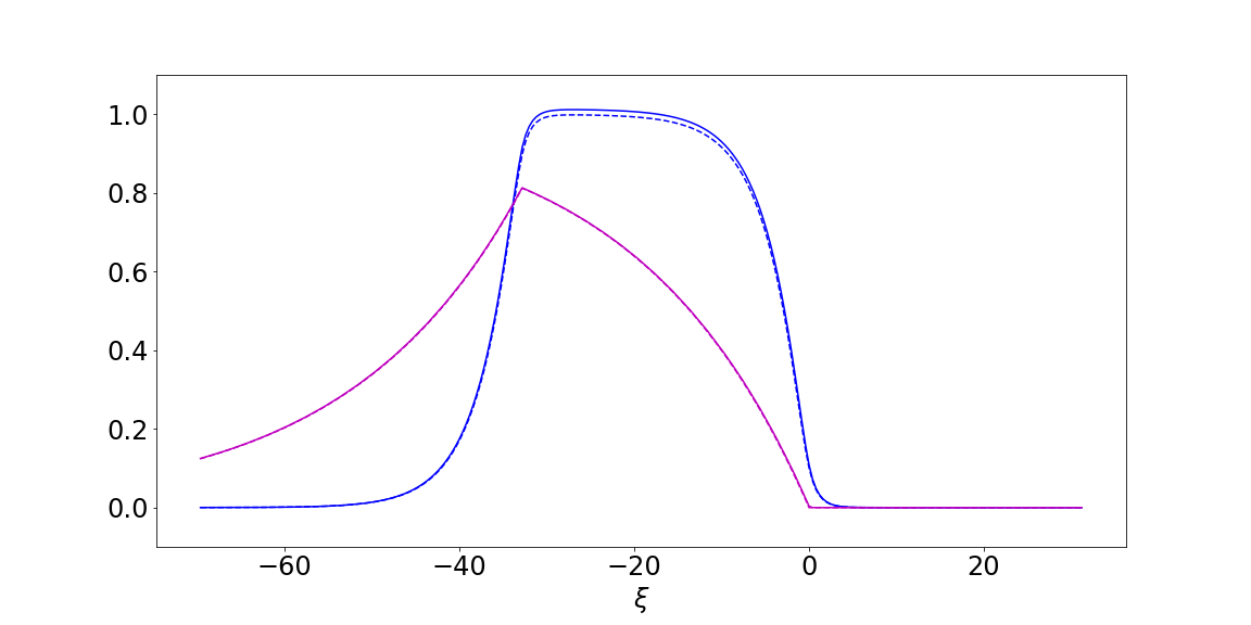
The results are not perfect, but suggest we have the correct analytical solution and some numerical error. Presumably, our measurements for $c$ and $\Delta$ from the simulation are in error. Using our measurement for $c$ and instead computing $\Delta$ from our condition gives a dramatically different profile, as seen in Figure 2, below.
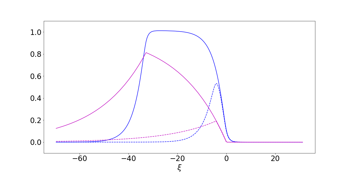
Using the measured value of $\Delta$ instead, proves unfruitful. In Figure 3 we plot the right-hand-side of the condition on $c$, as a function of $c$ and observe that it has roots near $c\approx 2, 4$. The root near $c \approx 4$ appears to be the stable one from our simulations. Unfortunatly, this function is quite ill-conditioned near this root for these particular parameters.
Correction: This funtion is not ill-conditioned near the root at $c \approx 4$. It is in fact very well conditioned as the derivative is quite large. The computation for $\Delta$, however, is very sensitive to the value of $c$ when $c \to 4$ leading to difficulties in computing the correct profile. See report 2021-06-17 for further discussion.

It may behoove us to find some sensible choice of parameters that allows for more precise numerics. In the meantime, here are numerical functions for generating traveling wave solutions.
def Unum(ξ, μ, α, γ, θ, Δ, c):
    return (1.0/2.0)*(1 - np.exp(-Δ))*np.exp(-ξ)*(lambda input: np.heaviside(input,0.5))(ξ)/(μ*c + 1) + ((1.0/2.0)*(-np.exp(Δ)/(μ*c - 1) + 1.0/(μ*c - 1))*np.exp(ξ) + (( lambda base, exponent: base**exponent )(μ, 2)*( lambda base, exponent: base**exponent )(c, 2)*np.exp(Δ/(μ*c)) - ( lambda base, exponent: base**exponent )(μ, 2)*( lambda base, exponent: base**exponent )(c, 2) - 1.0/2.0*μ*c + θ*(( lambda base, exponent: base**exponent )(μ, 2)*( lambda base, exponent: base**exponent )(c, 2) - 1) + (1.0/2.0)*(μ*c - 1)*np.exp(-Δ) + 1.0/2.0)*np.exp(ξ/(μ*c))/(( lambda base, exponent: base**exponent )(μ, 2)*( lambda base, exponent: base**exponent )(c, 2) - 1))*(lambda input: np.heaviside(input,0.5))(-Δ - ξ) + ((θ + (-( lambda base, exponent: base**exponent )(μ, 2)*( lambda base, exponent: base**exponent )(c, 2) - 1.0/2.0*μ*c + ((1.0/2.0)*μ*c - 1.0/2.0)*np.exp(-Δ) + 1.0/2.0)/(( lambda base, exponent: base**exponent )(μ, 2)*( lambda base, exponent: base**exponent )(c, 2) - 1))*np.exp(ξ/(μ*c)) + 1 - 1.0/2.0*np.exp(-Δ)*np.exp(-ξ)/(μ*c + 1) + (1.0/2.0)*np.exp(ξ)/(μ*c - 1))*(lambda input: np.heaviside(input,0.5))(-ξ)*(lambda input: np.heaviside(input,0.5))(Δ + ξ)

def Anum(ξ, μ, α, γ, θ, Δ, c):
    return γ*(1 - np.exp(ξ/(α*c)))*(lambda input: np.heaviside(input,0.5))(-ξ)*(lambda input: np.heaviside(input,0.5))(Δ + ξ) + γ*(np.exp(Δ/(α*c)) - 1)*np.exp(ξ/(α*c))*(lambda input: np.heaviside(input,0.5))(-Δ - ξ)
Wave Response Simulations
Figure 4 shows the traveling wave (with parameters given above) responding to a stimulus of $I(x,t) = \delta(t-t_0) 0.05$. As expected, the limiting effect is to advance the wave forward.
SymPy Bug
I spent quite a bit of time debugging my code before I found what appears to be an error in SymPy's integration subroutine. When I ask Sympy to integrate, for example $\int\limits_{-\Delta}^0 H(x-y)e^{y-x} \ dy$ it gives an incorrect result when the symbol $\Delta$ is initialized with positive=True. I have submitted a bug report and in the meantime, I integrated the forcing term by hand.