June 10^th, 2021

We have found an asymptotic approximation of the wave reponse function, though there is more work to be done determining the dimension of the null-space of the adjoint operator. The example that we have been simulating certainly has a one-dimensional null-space, though the particulars of that problem allow for a solution to be found. Comparison to simulations has proven difficult due to the inaccuracies in measuring the wave speed and front locations. We have outlined these difficulties here and proposed several possible solutions.

To-Do List Snapshot

Investigate wave-response function.

Spatially homogeneous pulse.
Spatially homogeneous, temporally finite.
Local pulses.

Wave-train Analysis

Search the literature.
Find periodic solutions.
Compare frequency to a pair of pulses.

Reading

Coombes 2004.
Folias & Bressloff 2005.
Faye & Kilpatrick 2018.

Wave Response: Adjoint Method

Beginning with the model $$\begin{align*} \mu u_t &= -u + \int_\RR w(x,y) f\big[ u(y,t) - a(y,t) \big] \ dy + \epsilon I(\xi, t) \\ \alpha a_t &= -a + \gamma \int_\RR w(x,y) f\big[ u(y,t) - a(y,t) \big] \ dy \end{align*}$$

We convert to $\xi$-$t$ coordinates via the mappings $x-ct \mapsto \xi$ and $t \mapsto t$ $$\begin{align*} -c\mu u_\xi + \mu u_t &= -u + \int_\RR w(\xi,y) f\big[ u(y,t) - a(y,t) \big] \ dy + \epsilon I(\xi, t) \\ -c\alpha a_\xi + \alpha a_t &= -a + \gamma \int_\RR w(\xi,y) f\big[ u(y,t) - a(y,t) \big] \ dy. \end{align*}$$

Then we make the asymptotic approximation $$\begin{align*} u(\xi, t) &= U(\xi - \epsilon \nu(t)) + \epsilon u_1(\xi, t) + \OO(\epsilon^2) \\ a(\xi, t) &= A(\xi - \epsilon \eta(t)) + \epsilon a_1(\xi, t) + \OO(\epsilon^2). \end{align*}$$ giving us $$\begin{align*} -c\mu (U_\xi + \epsilon \partial_\xi u_{1}) + \mu (-\epsilon \nu_t U_\xi + \epsilon \partial_t u_{1}) &= -U -\epsilon u_1 + \int_\RR w(\xi,y) \bigg[ f\big(U(y) - A(y)\big) + \epsilon f'(U-A)(u_1 - a_1) \bigg] \ dy + \epsilon I(\xi, t) + \OO(\epsilon^2)\\ -c\alpha (A_\xi + \epsilon \partial_\xi a_{1}) + \alpha (-\epsilon \eta_t A_\xi + \epsilon \partial_t a_{1}) &= -A - \epsilon a_1+ \gamma \int_\RR w(\xi,y) \bigg[ f\big(U(y) - A(y)\big) + \epsilon f'(U-A)(u_1 - a_1) \bigg] \ dy + \OO(\epsilon^2)\\ \end{align*}$$

Collecting the $\OO(1)$ terms, we have $$\begin{align*} -c\mu U_\xi &= -U + \int_\RR w(\xi, y) f\big[ U(y) - A(y) \big] \ dy \\ -c\alpha A_\xi &= -A + \gamma \int_\RR w(\xi, y) f\big[U(y) - A(y) \big] \ dy, \end{align*}$$ and thus $U$ and $A$ are the profiles of stable traveling pulses.

Collecting the $\OO(\epsilon)$ terms, we have $$\begin{align*} \mu \partial_t u_1 + u_1 - \mu c\partial_\xi u_1 - \int_\RR w(\xi, y) f'\big(U(y)-A(y)\big) \big(u_1(y,t) - a_1(y,t)\big) \ dy &= -\mu U_\xi \nu_t + I \\ \alpha \partial_t a_1 + a_1 - \alpha c \partial_\xi a_1 - \gamma \int_\RR w(\xi, y) f'\big(U(y)-A(y)\big) \big(u_1(y,t) - a_1(y,t)\big) \ dy &= -\alpha A_\xi \eta_t \end{align*}$$ or in vector form $$\begin{align*} \begin{bmatrix}\mu&0\\0&\alpha\end{bmatrix} \vecu_t + \underbrace{\vecu - c\begin{bmatrix}\mu&0\\0&\alpha\end{bmatrix} \vecu_\xi - \begin{bmatrix}1&-1\\ \gamma&-\gamma\end{bmatrix} \int_\RR w(\xi,y)f'\big(U(y) - A(y)\big) \vecu(y) \ dy}_{\LL \vecu} &= \begin{bmatrix}-\mu U_\xi \nu_t + I \\ -\alpha A_\xi \eta_t \end{bmatrix} \end{align*}$$ with $\vecu^T = [u_1, a_1]$.

Correction: The right-hand-side vector should be $$ \begin{bmatrix} \mu U_\xi \nu_t + I \\ \alpha A_\xi \eta_t \end{bmatrix} $$ A similar error was made in the computation of $\nu(t)$ below, which lead to the correct result.

Assume that a bounded solution will exist if the right-hand-side is orthogonal to the null-space of $$ \LL^* \vecv = \vecv + c \begin{bmatrix}\mu&0\\0&\alpha\end{bmatrix} \vecv_\xi - f'\big(U(\xi) - A(\xi)\big) \begin{bmatrix}1&\gamma \\ -1 &-\gamma\end{bmatrix} \int_\RR w(y, \xi) \vecv(y) \ dy. $$

We begin by defining the matrices $$ M_1 = \begin{bmatrix}\mu&0\\0&\alpha\end{bmatrix}, \qquad \text{ and } \qquad M_2 = \begin{bmatrix}1&-1\\ \gamma&-\gamma\end{bmatrix}, $$ for convenience. Then we have $$ \begin{align*} \langle \LL \vecu, \vecv \rangle &= \int_\RR \LL \vecu \cdot \vecv \ d\xi \\ &= \int_\RR \vecv^T \vecu - c\vecv^T M_1 \vecu_\xi - \vecv^T M_2 \int_\RR w(\xi, y) f'\big(U(y) - A(y)\big) \vecu(y) \ dy \ d\xi \\ &= \int_\RR \vecv^T \vecu \ d\xi - c \int_\RR \vecv^T M_1 \vecu_\xi \ d\xi - \int_\RR \int_\RR w(\xi, y) f'\big(U(y) - A(y)\big) \ \vecv^T M_2 \vecu(y) \ dy \ d\xi \\ &= \int_\RR \vecv^T \vecu \ d\xi - c\vecv^TM_1\vecu \bigg|_{-\infty}^\infty + c\int_\RR \vecv^T_\xi M_1 \vecu \ d\xi - \int_\RR \int_\RR w(\xi, y) f'\big(U(y) - A(y)\big) \ \vecv^T(\xi) M_2 \vecu(y) \ dy \ d\xi \tag{IBP} \\ &= - c\vecv^TM_1\vecu \bigg|_{-\infty}^\infty + \int_\RR \vecv^T \vecu \ d\xi + c\int_\RR \vecv^T_\xi M_1 \vecu \ d\xi - \int_\RR \int_\RR w(y, \xi) f'\big(U(\xi) - A(\xi)\big) \ \vecv^T(y) M_2 \vecu(\xi) \ dy \ d\xi \tag{change of varialbes} \\ &= - c\vecu^TM_1^T\vecv \bigg|_{-\infty}^\infty + \int_\RR \vecu^T \vecv \ d\xi + c\int_\RR \vecu^T M_1^T \vecv_\xi \ d\xi - \int_\RR \int_\RR w(y, \xi) f'\big(U(\xi) - A(\xi)\big) \ \vecu^T(\xi) M_2^T \vecv(y) \ dy \ d\xi \tag{transpose of scalars} \\ &= - c\vecu^TM_1^T\vecv \bigg|_{-\infty}^\infty + \int_\RR \vecu^T\bigg( \vecv + c M_1^T \vecv_\xi - f'\big(U(\xi) - A(\xi)\big)\int_\RR w(y, \xi) \ M_2^T \vecv(y) \ dy \ \bigg)d\xi. \end{align*}$$ Assuming that $c\vecu^TM_1^T\vecv \bigg|_{-\infty}^\infty = 0$ this gives us $$ \LL^* \vecv = \vecv + c M_1^T \vecv_\xi - f'\big(U(\xi) - A(\xi)\big)\int_\RR w(y, \xi) \ M_2^T \vecv(y) \ dy $$ or $$ \LL^* \vecv = \vecv + c \begin{bmatrix}\mu&0\\0&\alpha\end{bmatrix} \vecv_\xi - f'\big(U(\xi) - A(\xi)\big)\int_\RR w(y, \xi) \begin{bmatrix}1&\gamma \\ -1 &-\gamma\end{bmatrix} \vecv(y) \ dy. $$

Let $\vecv = [v_1, v_2]^T \in \text{Null}(\LL^*)$. We require $$\begin{align*} \vec{0} &= \left\langle \vecv, \begin{bmatrix}-\mu U_\xi \nu_t + I \\ -\alpha A_\xi \eta_t \end{bmatrix} \right\rangle \\ &= \int_\RR -\mu U_\xi \nu_t v_1(\xi) + v_1(\xi, t)I(\xi, t) -\alpha A_\xi \eta_t v_2(\xi,t) \ d\xi \\ \left( \int_\RR \mu U_\xi v_1(\xi) \ d\xi \right) \nu_t + \left( \int_\RR \alpha A_\xi v_2(\xi) \ d\xi \right) \eta_t&= \int_\RR v_1(\xi) I(\xi, t) \ d\xi \end{align*}$$

We can find $\nu_t$ and $\eta_t$ as the solution to the set of equations $$ \left( \int_\RR \mu U_\xi v_1(\xi) \ d\xi \right) \nu_t + \left( \int_\RR \alpha A_\xi v_2(\xi,t) \ d\xi \right) \eta_t = \int_\RR v_1(\xi) I(\xi, t) \ d\xi $$ for all vectors $\vecv = [v_1, v_2]^T \in \text{Null}(\LL^*)$.

We believe this adjoint has a one-dimensional null-space, due to the rank-deficiency of the coupling matrix. This leaves us with not enough information to solve for both $\nu$ and $\eta$. It would, perhaps, be reasonable to assume that $\nu = \eta$. Interestingly, the point is moot in the following example.

Heaviside Firing-rate with Exponential Weight

In the case of $$\begin{align*} f(\cdot) &= H(\cdot - \theta) & w(x,y) &= \tfrac{1}{2} e^{-|x-y|} \end{align*}$$ we find $$\begin{align*} v_1(\xi) &= \alpha H(\xi) e^{-\xi/c\mu} \\ v_2(\xi) &= -\mu H(\xi) e^{-\xi/c\alpha}. \end{align*}$$

We can compute the null-space as follows: $$\begin{align*} \vec{0} &= \LL^* \vecv \\ &= \vecv + c \begin{bmatrix}\mu&0\\0&\alpha\end{bmatrix} \vecv_\xi - \frac{d}{d \xi}\bigg[ H\big( U(\xi) - A(\xi) \big) \bigg] \begin{bmatrix}1&\gamma \\ -1 &-\gamma \end{bmatrix} \int_\RR e^{-|y-\xi |}\vecv(y) \ dy \\ &= \vecv + c \begin{bmatrix}\mu&0\\0&\alpha\end{bmatrix} \vecv_\xi - \frac{\delta(\xi)}{U'(0) - A'(0)} \begin{bmatrix}1&\gamma \\ -1 &-\gamma \end{bmatrix} \int_\RR e^{-|y|}\vecv(y) \ dy \\ \vecv + c\begin{bmatrix}\mu&0\\0&\alpha\end{bmatrix} \vecv_\xi &= \frac{\delta(\xi)}{U'(0) - A'(0)} \begin{bmatrix}1&\gamma \\ -1 &-\gamma \end{bmatrix} \int_\RR e^{-|y|}\vecv(y) \ dy \\ \vecv_\xi + \frac{1}{c} \begin{bmatrix}\mu&0\\0&\alpha\end{bmatrix}^{-1} \vecv &= \frac{\delta(\xi)}{U'(0) - A'(0)} \begin{bmatrix}\frac{1}{\mu} &\frac{\gamma}{\mu} \\ -\frac{1}{\alpha} &-\frac{\gamma}{\alpha} \end{bmatrix} \int_\RR e^{-|y|}\vecv(y) \ dy \\ \left[ \exp\left(\frac{\xi}{c} \begin{bmatrix}\mu&0\\0&\alpha\end{bmatrix}^{-1} \right) \vecv \right]_\xi &= \exp\left(\frac{\xi}{c} \begin{bmatrix}\mu&0\\0&\alpha\end{bmatrix}^{-1} \right) \frac{\delta(\xi)}{U'(0) - A'(0)} \begin{bmatrix}\frac{1}{\mu} &\frac{\gamma}{\mu} \\ -\frac{1}{\alpha} &-\frac{\gamma}{\alpha} \end{bmatrix} \int_\RR e^{-|y|}\vecv(y) \ dy \\ \exp\left(\frac{\xi}{c} \begin{bmatrix}\mu&0\\0&\alpha\end{bmatrix}^{-1} \right) \vecv &= H(\xi) \left[ \exp\left(\frac{\xi}{c} \begin{bmatrix}\mu&0\\0&\alpha\end{bmatrix}^{-1} \right) \frac{1}{U'(0) - A'(0)} \begin{bmatrix}\frac{1}{\mu} &\frac{\gamma}{\mu} \\ -\frac{1}{\alpha} &-\frac{\gamma}{\alpha} \end{bmatrix} \int_\RR e^{-|y|}\vecv(y) \ dy \right]_{\xi = 0} \\ \exp\left(\frac{\xi}{c} \begin{bmatrix}\mu&0\\0&\alpha\end{bmatrix}^{-1} \right) \vecv &= H(\xi) \frac{1}{U'(0) - A'(0)} \begin{bmatrix}\frac{1}{\mu} &\frac{\gamma}{\mu} \\ -\frac{1}{\alpha} &-\frac{\gamma}{\alpha} \end{bmatrix} \int_\RR e^{-|y|}\vecv(y) \ dy. \end{align*}$$

The integral on the right-hand-side is some constant vector $$ \frac{1}{U'(0) - A'(0)} \int_\RR e^{-|y|}\vecv(y) \ dy = \begin{bmatrix} w_1 \\ w_2 \end{bmatrix} $$ so we have \begin{align*} \vecv(\xi) &= H(\xi) \exp\left(-\frac{\xi}{c} \begin{bmatrix}\mu&0\\0&\alpha\end{bmatrix}^{-1} \right) \begin{bmatrix}\frac{1}{\mu} &\frac{\gamma}{\mu} \\ -\frac{1}{\alpha} &-\frac{\gamma}{\alpha} \end{bmatrix} \begin{bmatrix} w_1 \\ w_2 \end{bmatrix}. \end{align*}

This constant matrix is rank 1 and thus the null-space of $\LL^*$ is one-dimensional. Fixing the arbitrary scaling of the null-vector, we arrive at $$\begin{align*} \vecv(\xi) &= H(\xi) \exp\left(-\frac{\xi}{c} \begin{bmatrix}\mu&0\\0&\alpha\end{bmatrix}^{-1} \right) \begin{bmatrix} \alpha \\ -\mu \end{bmatrix} \end{align*}$$ or equivalently $$\begin{align*} v_1(\xi) &= \alpha H(\xi) e^{-\xi/c\mu} \\ v_2(\xi) &= -\mu H(\xi) e^{-\xi/c\alpha}. \end{align*}$$

Conveniently, $A(\xi)$ and $v_2(\xi)$ are orthogonal, and thus we simplify to $$\begin{align*} \nu(t) &= \frac{ \int_0^t \int_\RR \alpha H(\xi) e^{-\xi/c\mu} I(\xi, \tau) \ d\xi \ d\tau}{\int_\RR \mu U_\xi \alpha H(\xi) e^{-\xi/c\mu} d\xi} \\ &= \frac{1}{\mu} \frac{\int_0^t \int_0^\infty e^{-\xi/c\mu} I(\xi, t) \ d\xi \ d\tau }{\int_\RR U_\xi e^{-\xi/c\mu} d\xi } \\ &= \frac{2(\mu c+1)}{\mu(e^{-\Delta}-1)} \frac{ \int_0^t \int_0^\infty e^{-\xi/c\mu} I(\xi, t) \ d\xi \ d\tau }{\int_\RR e^{-\xi(1+1/c\mu)} d\xi} \\ &= \frac{2(\mu c+1)}{\mu(1 - e^{-\Delta})} (1 + \tfrac{1}{c\mu}) \int_0^t \int_0^\infty e^{-\xi/c\mu} I(\xi, t) \ d\xi \ d\tau \\ &= \frac{2(\mu c+1)^2}{\mu^2 c (1 - e^{-\Delta})} \int_0^t \int_0^\infty e^{-\xi/c\mu} I(\xi, t) \ d\xi \ d\tau. \end{align*}$$

From the previous report we have that $1 - e^{-\Delta} = 2\theta(\mu c + 1)$ and thus we have $$ \nu(t) = \frac{\mu c+1}{\mu^2 c \theta} \int_0^t \int_0^\infty e^{-\xi/c\mu} I(\xi, t) \ d\xi \ d\tau $$

Spatially Homogeneous Stimulus

If we consider stimuli of the form $I(\xi, t) = I_0 \delta(t)$ then we have $$\begin{align*} \nu(t) &= \frac{\mu c+1}{\mu^3 c^2 \theta} I_0. \end{align*}$$

Correction: There is an error in the computation of this final integral. The Wave response function is actually given by $$\begin{align*} \nu(t) &= \frac{\mu c+1}{\mu \theta} I_0. \end{align*}$$

Numerical Difficulties

Ideally, we would compare our asymptotic approximation of the wave repsonse function to numerical simulations. This has proven to be numerically difficult. To accurately measure the wave response function for a given simulation, we must be able to measure the pulse speed accurately. Figure 1 shows the measured speed, as determined by the approximate front locations over time. While the forward front of the pulse appears to have a relatively stable speed, the rear of the pulse seems to be oscillating.

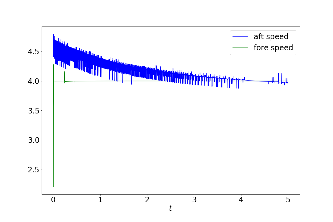
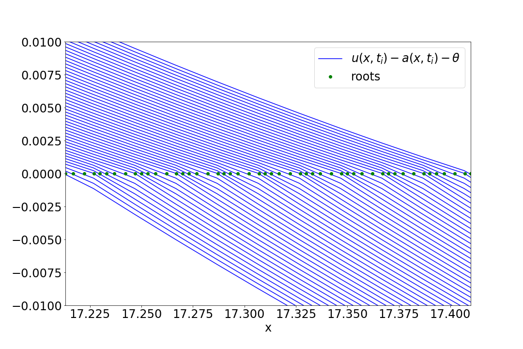
**Fig 1.** The measured speed of the fore and aft fronts. (Slope of secant lines for points separated by 50 time steps. Parameters are given in Figure 1).

Figure 2 shows the solution $u(x,t)-a(x,t)$ at consecutive time-steps. Far from the front we see that the solution is clearly advecting, however near the front we are observing oscillations in the speed that compress and expand the distance between consecutive time-steps. These oscillations are in the solutions themselves rather than artifacts of the root-finding process.

Additionally, that the traveling solution is piece-wise suggests that this naive interpolation will be at most $\OO(h)$ accurate - no better than simply finding an argmin of $|u - a - \theta|$.

**Fig 2.** The solution $u(x,t) - a(x,t) - \theta$ for 50 consecutive time steps after the pulse has stabilized as well as an approximation of the front location (quartic interpolation). We see the solutions are not smooth causing difficulties in measuring the location of the front to a reasonable degree of accuracy. The parameters are the same as the simulations in the previous weeks: $\mu = 1, \alpha = 5, \gamma = 1, \theta = 0.1$. The simulation was initiallized with our previously calculated traveling-pulse solution (based on the poorly approximated pulse speed and width) and allowed to stabilze for 4300 time steps at a temporal resolution of $\Delta t = 10^{-3}$ and a spatial resolution of $\Delta x = 2\times 10^{-2}$.

Measuring the pulse widths is marred by this inaccuracy in the front locations as well. Figure 3 shows the measurments over the course of the simulation on two time-scales. The finer time-scale shows that the apparant difference between the front locations seems to oscilate rappidly.

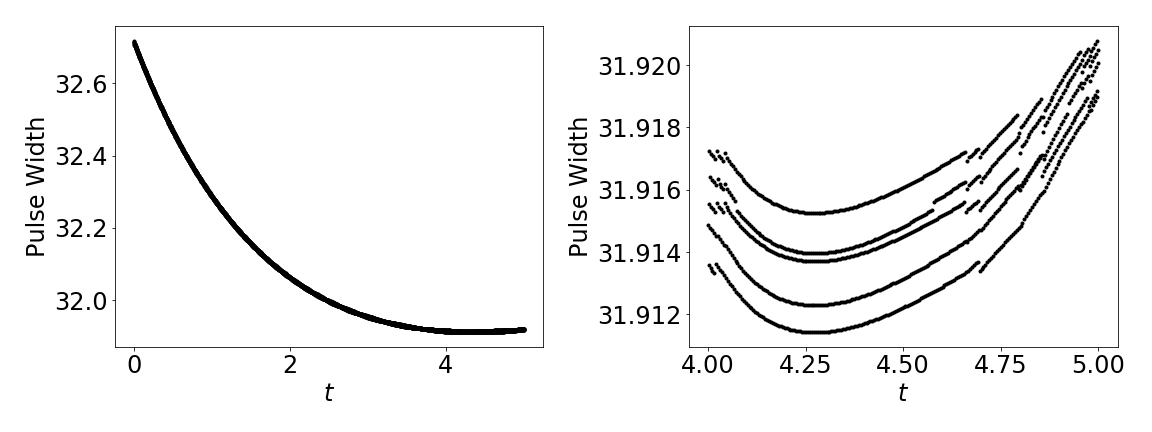
**Fig 3.** Measurements of the pulse width shown on two time scales for clarity. In the region near $t=4.25$ we see five distinct curves.

It was curious that. in Figure 1, the oscillations in the aft speed seemed to vanish near $t\approx 4.25$. This is explained by the finer time-scale in Figure 3, as it appears the frequency of the ocilations is aliased - there are clearly 5 curves in this region, and our measurment of the pulse speed took samples spaced 50 indices appart.

Going Forward

Though it is not included here, we did attempt to find parameter regimes that were more well-conditioned, without success. We tried arbitrarily selecting the wave speed and using the first condition $0 = (2\theta(\mu c+1)-1)e^\Delta + 1$ (which relies on fewer of the parameters) to determine the pulse width, and then use the second condition to determine one of the unknown parameters, however, the solution would no longer sustain traveling pulses. the solutions would default to traveling front solutions. We may need to investigate stability conditions to proceed in this way.

That these oscillations in front locations are an artifact of the simulations themselves suggest that we revisit the numerics of the simulations. The piece-wise profile suggests that they are not smooth in space, and that the computation of the convolution is only to first order. An analytic evaluation of the convolution should be possible if we can accurately calculate the front locations. Perhaps if we use this from the beginning, the oscillations will not be present, and the traveling pulse solution will maintain a higher degree of spatial smoothness over time.

It could also be interesting to try a piece-wise interpolation. We can perhaps assume that the solution is smooth on either side of the front, and that the kink occurs at threshold-crossing. We can enforce continuity (and possibly some degree of smoothness) and solve for the location of the kink. We should have enough equations, though they will be non-linear in the location variable. Still, the problem appears well conditioned, so perhaps it will not be too difficult. The error analysis of such an interpolation technique would be interesting more generally.