August 8th, 2022
We find an asymptotic approximation to the wave response function for the traveling front case.
Traveling Front Solution
We find the traveling front solution to be of the form \begin{align*} Q(\xi) &= \begin{cases} A_1 + A_2 e^{\frac{1 + \alpha\beta}{\alpha c} \xi} & \xi < 0 \\ 1 & \xi \ge 0 \end{cases} \\ U(\xi) &= \begin{cases} A_3 + A_4 e^{\xi} + A_5 e^{\frac{1}{\mu c}\xi} + A_6 e^{\frac{1 + \alpha\beta}{\alpha c} \xi} & \xi < 0 \\ A_7 e^{-\xi} & \xi \ge 0 \end{cases} \end{align*} where the constants $A_1, \dots, A_7$ depend on the model parameters $\alpha, \mu, \beta, \theta$ and the front speed $c$. The speed itself is given by equation $$\begin{align*} \theta = A_7 = \frac{\alpha c + 1}{2(\mu c + 1)(\alpha \beta + \alpha c + 1)} \end{align*}$$ which is identical to the condition from Kilpatrick Bressloff 2010 despite the inclusion of a hyper-polarizing adaptation variable.
This is consistent with expectations. In both cases, the active region remains super-threshold. The threshold crossing is advancing into a region where the $\theta$ is constant since the adaptation variable, $a(x,t) = 0$. The only difference is the condition for a traveling pulse to exist: $\theta > \frac{1}{1+\alpha \beta} = \lim\limits_{\xi \to -\infty}Q(\xi)$, which does not include an adaptation strength variable $\gamma$. It is consistent with their condition in the case of $\gamma = 0$.
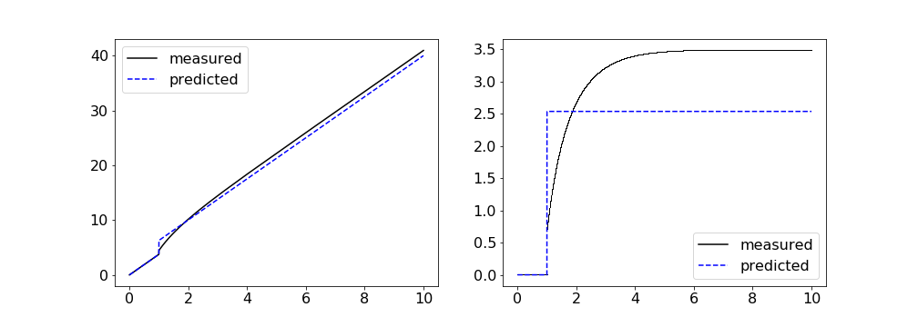
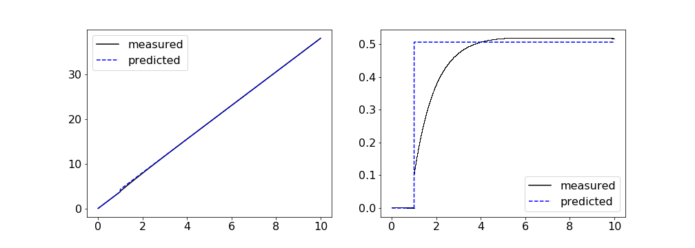
The animation below shows a simulation of the model initialized with the traveling pulse solution. As expected, it simply advects to the right with a constant speed. Model parameters are as follows $$\begin{align*} \mu &= 1 & \alpha &= 20 \\ \beta &= 0.2 & \theta &= 0.1 \\ c &= 3.75. \end{align*}$$
Wave Response
From our wave response derivation, we seek a nullspace $[v_1\ v_2]^T$ satisfying \begin{align*} -c\mu v_1' - v_1 &= -\frac{\delta(\xi)}{|U'(\xi)|}Q\big[(w * v_1) + \alpha\beta v_2) \big] \\ -c\alpha v_2' - v_2 &= H(-\xi)\big(-(w*v_1) + \alpha\beta v_2\big). \end{align*} Choose the normalization such that the jump-discontinuity in $v_1$ has magnitude 1. Then we have $v_1(\xi) = H(\xi)e^{-\frac{1}{c\mu}\xi}$. This gives \begin{align*} w * v_1 &= \int_0^\infty \frac{1}{2}e^{-|\xi - y|}e^{-\frac{1}{c\mu}y} \ dy \\ \end{align*} If $\xi > 0$ then $-c\alpha v_2' - v_2 = 0$ and $v_2(\xi) = A_8 e^{-\frac{1}{c\alpha}\xi}$. If $\xi < 0$ then $\xi - y < 0$ and \begin{align*} (w * v_1) &= \int_0^\infty \frac{1}{2}e^{\xi} e^{-y}e^{-\frac{1}{c\mu}y} \ dy \\ &= \frac{1}{2}e^{\xi} \int_0^\infty e^{-\frac{1+c\mu}{c\mu} y} \ dy \\ &= \frac{c \mu}{2(1+c\mu)}e^{\xi} \end{align*} so we have \begin{align*} -c\alpha v_2' - (1+\alpha\beta)v_2 &= -\frac{c \mu}{2(1+c\mu)}e^{\xi} \\ v_2' + \frac{1+\alpha \beta}{c\alpha} v_2 &= \frac{\mu}{2\alpha (1+c\mu)} e^{\xi} \\ \big[ v_2 e^{\frac{1+\alpha\beta}{c\alpha}\xi} \big]' &= \frac{\mu}{2\alpha (1+c\mu)} e^{\frac{1+\alpha\beta + c\alpha}{c\alpha}\xi} \\ v_2 e^{\frac{1+\alpha\beta}{c\alpha}\xi} &= A_8 + \frac{c\mu}{2 (1+c\mu)(1+\alpha\beta+c\alpha)} e^{\frac{1+\alpha\beta + c\alpha}{c\alpha}\xi} \\ v_2(\xi) &= A_8 e^{-\frac{1+\alpha\beta}{c\alpha} \xi} + \frac{c\mu}{2 (1+c\mu)(1+\alpha\beta+c\alpha)} e^{\xi}. \end{align*} To remain bounded, $A_8 = 0$ and we have $$ v_2(\xi) = \frac{c\mu}{2 (1+c\mu)(1+\alpha\beta+c\alpha)} e^{\xi} \qquad \text{ if } \xi < 0. $$ Since $Q' = 0$ when $\xi > 0$, this is sufficient to calculate the approximate wave response.
In particular, \begin{align*} \int_\mathbb{R} U' v_1 \ d \xi &= \int_0^\infty -\theta e^{-\xi}e^{-\frac{1}{c\mu}\xi} \ d\xi \\ &= -\theta\frac{c\mu}{1+c\mu} \\ \int_{\mathbb{R}} Q' v_2 \ d\xi &= \int_{-\infty}^0 \underbrace{A_2}_{\frac{\alpha\beta}{1+\alpha\beta}} \frac{1+\alpha\beta}{\alpha c}e^{\frac{1+\alpha\beta}{\alpha c} \xi} \frac{c\mu}{2 (1+c\mu)(1+\alpha\beta+c\alpha)} e^{\xi} \ d\xi \\ &= \int_{-\infty}^0\frac{\mu \beta}{2 (1+c\mu)(1+\alpha\beta + c\alpha)} e^{\frac{1+\alpha\beta + c\alpha}{c\alpha} \xi} \ d\xi \\ &= \frac{\mu \alpha \beta c}{2(1+c\mu)(1+\alpha\beta + c\alpha)^2}. \end{align*} Thus \begin{align*} \nu(t) &= \frac{\int_0^\infty e^{-\frac{1}{c\mu}\xi} \int_0^t I(\xi, \tau) \ d\tau \ d\xi}{ \frac{\theta c \mu^2}{1+c\mu} - \frac{\mu \alpha^2 \beta c}{2(1+c\mu)(1+\alpha\beta + c\alpha)^2}}. \end{align*}