May 27th, 2021
We simulate the modified KB10 model (perhaps we will call it the $\beta$-null regime of the KB10 model) and find parameters that appear to admit traveling pulse solutions. We analyzed equations 3.30-3.31 from Kilpatrick & Bressloff 2010 in this case, but they appear inconsistent with observations. Perhaps the assumption that $\beta \ne 0$ was essential in their derivation. We may have to re-derive the traveling-pulse solution from scratch.
To-Do List Snapshot
Simulate the KB10 model, but without $q$. Find parameters that admit traveling pulse solutions.- Analytically find the traveling pulse/front solutions.
- Investigate wave-response function.
- Spatially homogeneous pulse.
- Spatially homogeneous, temporally finite.
- Local pulses.
- Wave-train Analysis
- Search the literature.
- Find periodic solutions.
- Compare frequency to a pair of pulses.
Experiment with colliding pulses.- Reading
- Coombes 2004.
- Folias & Bressloff 2005.
- Faye & Kilpatrick 2018.
Modified KB10 Simulation
What we are calling the modifed KB10 model is the model from Kilpatrick & Bressloff 2010 (KB10) but with the synaptic depression ($q$) removed. This is equivalent to setting $\beta = 0$ and initializing $q = 1$ in their model. The result is then $$\begin{align*} \mu u_t &= -u + \int_{-\infty}^\infty w(x,x^\prime) f( u(x^\prime,t) - a(x^\prime,t)) \ dx^\prime \\ \alpha a_t &= -a + \gamma f(u - a). \end{align*}$$ Note that we have re-labeled the parameters $\epsilon \to \alpha$ and the old $\alpha$ is not present.
With the removal of the synaptic depression variable, we will need to find new parameter-sets that admit traveling wave solutions. In particular, in KB10 with their choice of parameters, the synaptic depression appeared to be the primary restorative force, with hyperpolarizing adaptation current ($a$) playing a minor role. With our removal of the synaptic depression we will need to tune the parameters so that the hyperpolarizing adaptation current can provide sufficient restoration. This suggests increasing $\gamma$. Below, Figure 1 does exactly this and we indeed have a traveling pulse.
Figure 2 (below) shows the same parameter choices, but with the initial conditions set to create two pulses traveling in opposite directions. As predicted, they simply annihilate eachother. Since the traveling pulse solutions to the modified KB10 model are unique (as it is a special case of the KB10 model) there are essentially no other configurations to test. I don't think that there is anything interesting to study for colliding pulses in one dimension.
Traveling Pulse Solutions
Since we are working with a special case of the KB10 model, should be able to re-use the analysis from Kilpatrick & Bressloff 2010. In particular, their Equations 3.30-31 give that our wave speed $c$ and pulse width $\Delta$ are given as the solution to the following system (derivation below) $$\begin{align*} \Delta &= \log{\left(\frac{1}{- 2 \theta \left(c + 1\right) + 1} \right)}\\ 0 &= \gamma \left(\left(- 2 \theta \left(c + 1\right) + 1\right)^{\frac{\alpha}{c}} - 1\right) + \frac{- 2 \theta c + c^{2} \left(- 2 \theta - \left(- 2 \theta \left(c + 1\right) + 1\right)^{\frac{1}{c}} + 1\right)}{c^{2} - 1}. \end{align*}$$
We begin with $$\begin{align*} 0 &= K_{0} - K_{1} e^{- \Delta} - K_{2} e^{- \Delta} e^{\frac{\Delta \left(- \alpha \beta - 1\right)}{\alpha c}} - \theta\\ 0 &= L_{0} + L_{1} e^{- \Delta} + L_{2} e^{\frac{\Delta \left(- \alpha \beta - 1\right)}{\alpha c}} - L_{3} e^{- \frac{\Delta}{c}} + \gamma e^{- \frac{\Delta}{\epsilon c}} - \theta\\ K_{0} &= \frac{\alpha c + 1}{\left(2 c + 2\right) \left(\alpha \beta + \alpha c + 1\right)}\\ K_{1} &= \frac{1}{\left(2 c + 2\right) \left(\alpha \beta + 1\right)}\\ K_{2} &= \frac{\alpha^{2} \beta c}{\left(2 c + 2\right) \left(\alpha \beta + 1\right) \left(\alpha \beta + \alpha c + 1\right)}\\ L_{0} &= - \gamma + \frac{c + \frac{1}{2}}{\left(c + 1\right) \left(\alpha \beta + 1\right)}\\ L_{1} &= \frac{\alpha c - 1}{\left(2 c - 2\right) \left(- \alpha \beta + \alpha c - 1\right)}\\ L_{2} &= \frac{\alpha^{4} \beta c^{2}}{\left(\alpha \beta + 1\right) \left(\alpha^{2} c^{2} - \left(\alpha \beta + 1\right)^{2}\right) \left(- \alpha \beta + \alpha - 1\right)} - \frac{\alpha^{2} \beta c}{2 \left(c + 1\right) \left(\alpha \beta + 1\right) \left(\alpha \beta + \alpha c + 1\right)}\\ L_{3} &= \frac{\frac{\alpha^{4} \beta c^{2}}{\left(\alpha^{2} c^{2} - \left(\alpha \beta + 1\right)^{2}\right) \left(- \alpha \beta + \alpha - 1\right)} + 1}{\alpha \beta + 1} + \frac{\alpha^{2} c^{2} \left(\beta + 1\right) - \alpha \beta - 1}{\left(c^{2} - 1\right) \left(\alpha^{2} c^{2} - \left(\alpha \beta + 1\right)^{2}\right)}. \end{align*}$$ Then set $\beta=0$ to obtain $$\begin{align*} 0 &= K_{0} - K_{1} e^{- \Delta} - K_{2} e^{- \Delta} e^{- \frac{\Delta}{\alpha c}} - \theta\\ 0 &= L_{0} + L_{1} e^{- \Delta} + L_{2} e^{- \frac{\Delta}{\alpha c}} - L_{3} e^{- \frac{\Delta}{c}} + \gamma e^{- \frac{\Delta}{\epsilon c}} - \theta\\ K_{0} &= \frac{1}{2 \left(c + 1\right)}\\ K_{1} &= \frac{1}{2 c + 2}\\ K_{2} &= 0\\ L_{0} &= - \gamma + \frac{c + \frac{1}{2}}{c + 1}\\ L_{1} &= \frac{1}{2 c - 2}\\ L_{2} &= 0\\ L_{3} &= 1 + \frac{1}{c^{2} - 1}. \end{align*}$$ Substituting, we find $$\begin{align*} 0 &= - \theta - \frac{e^{- \Delta}}{2 c + 2} + \frac{1}{2 \left(c + 1\right)}\\ 0 &= \gamma \left(-1 + e^{- \frac{\Delta}{\epsilon c}}\right) - \theta + \frac{c}{c + 1} - e^{- \frac{\Delta}{c}} - \frac{1}{c^{2} e^{\frac{\Delta}{c}} - e^{\frac{\Delta}{c}}} + \frac{e^{- \Delta}}{2 c - 2} + \frac{1}{2 \left(c + 1\right)}. \end{align*}$$ Solving the first equation for $e^{-\Delta}$ and substituting, we obtain $$\begin{align*} e^{- \Delta} &= - 2 \theta c - 2 \theta + 1\\ 0 &= \gamma \left(\left(- 2 \theta c - 2 \theta + 1\right)^{\frac{1}{\epsilon c}} - 1\right) - \theta + \frac{c}{c + 1} - \left(- 2 \theta c - 2 \theta + 1\right)^{\frac{1}{c}} - \frac{1}{c^{2} \left(- 2 \theta c - 2 \theta + 1\right)^{- \frac{1}{c}} - \left(- 2 \theta c - 2 \theta + 1\right)^{- \frac{1}{c}}} + \frac{- 2 \theta c - 2 \theta + 1}{2 c - 2} + \frac{1}{2 \left(c + 1\right)}. \end{align*}$$ Rearranging, we arrive at a one-dimensional root finding problem for $c$, and some simple substitution for $\Delta$ $$\begin{align*} \Delta &= \log{\left(\frac{1}{- 2 \theta \left(c + 1\right) + 1} \right)}\\ 0 &= \gamma \left(\left(- 2 \theta \left(c + 1\right) + 1\right)^{\frac{1}{\epsilon c}} - 1\right) + \frac{- 2 \theta c + c^{2} \left(- 2 \theta - \left(- 2 \theta \left(c + 1\right) + 1\right)^{\frac{1}{c}} + 1\right)}{c^{2} - 1}. \end{align*}$$ Converting to our parameter naming conventions $\epsilon \to 1/\alpha$ we have $$\begin{align*} \Delta &= \log{\left(\frac{1}{- 2 \theta \left(c + 1\right) + 1} \right)}\\ 0 &= \gamma \left(\left(- 2 \theta \left(c + 1\right) + 1\right)^{\frac{\alpha}{c}} - 1\right) + \frac{- 2 \theta c + c^{2} \left(- 2 \theta - \left(- 2 \theta \left(c + 1\right) + 1\right)^{\frac{1}{c}} + 1\right)}{c^{2} - 1}. \end{align*}$$
In order for $c$ and $\Delta$ to be real-valued, we require $c < \frac{1}{2\theta} - 1$. For our choice of parameters in the simulations above ($\gamma = 1, \theta = 0.1$) this suggests a maximum speed of $c_\text{max} = 4$. Unfortunatley, rootfinding attempts have been unsuccessful. Figure 3 below, shows a plot of the RHS of our expression, for which we seek a root. It appears that the function is bounded above by $-0.2$ and thus no root can exisit. This seems at odds with our simulation.
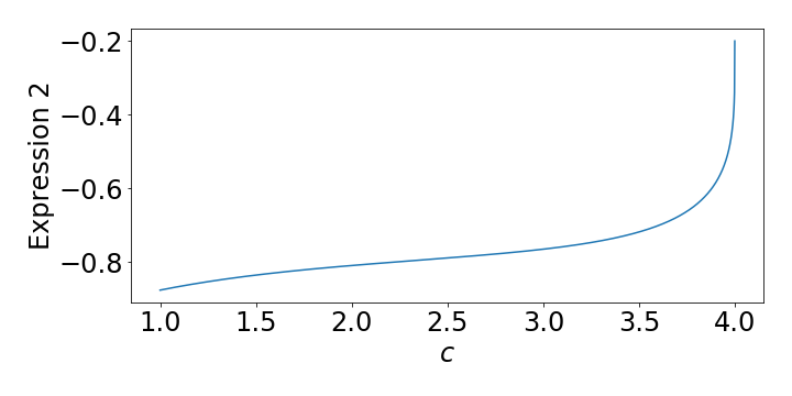
For reference, here is the generated code for the function depicted in Figure 3, above.
def c_implicit(c, γ, α, θ=0.1):
    return γ*(( lambda base, exponent: base**exponent )(-2*θ*(c + 1) + 1, α/c) - 1) + (-2*θ*c + ( lambda base, exponent: base**exponent )(c, 2)*(-2*θ - ( lambda base, exponent: base**exponent )(-2*θ*(c + 1) + 1, 1.0/c) + 1))/(( lambda base, exponent: base**exponent )(c, 2) - 1)