August 8th, 2023
We apply the new wave response differential equation to the problem of apparent motion and find and asymptotic prediction for the threshold of entrainment. The predicted threshold to entrain to an apparently moving square stimulus is the same as the threshold to entrain to an actually moving stimulus with amplitude multiplied by the proportion of time that the stimulus is present.
The Apparent Motion Stimulus
For the apparent motion experiment, we will select the stimulus to have certain properties. It is flashing, so it will be non-zero for a length of time $T_\text{on}$ and will be zero for a length of time $T_\text{off}$. During the on period, the stimulus will be localized and stationary. For this analysis, we will take the spatial profile of the stimulus to be a square pulse with rising edge at $\hat{y}-\Delta_y$ and falling edge at $\hat{y}$. We will call $T = T_\text{on} + T_\text{off}$ the period of the stimulus, and $\frac{1}{T}$ the frequency. Between successive on periods, the stimulus will shift forward by the fixed amount $(c + \Delta_c) T$, where $\Delta_c$ is the speed of the stimulus relative to the natural (unstimulated) pulse speed.
These criteria give the following formula for the activity stimulus $$ I_u(x, t) = I_{(\hat{y} - \Delta_y, \hat{y})}\left(x - \left\lfloor \frac{t}{T} \right\rfloor (c + \Delta_c)T \right) I_{(0, T_\text{on})}\left( t - \left\lfloor \frac{t}{T} \right\rfloor T \right). $$ We will restrict our analysis to the first period, which simplifies the stimulus to \begin{align*} I_u(x,t) = \begin{cases} I_{(\hat{y} - \Delta_y, \hat{y})}(x), & t < T_\text{on} \\ 0, & \text{else}. \end{cases} \\ I_u(\xi, t) = \begin{cases} I_{(\hat{y} - ct - \Delta_y, \hat{y} - ct)}(\xi), & t < T_\text{on} \\ 0, & \text{else}. \end{cases} \end{align*}
It is helpful to divide the scenario into several cases involving the position of the threshold crossing relative to the active region during the on-interval. We will consider the simplest case first. In the simplest case (Case 1) we will assume that the fore threshold crossing is in the support of the stimulus for the duration of the on interval. In the second case (Case 2) the stimulus jumps beyond the threshold crossing, but the period is long enough for the stimulus to catch up and enter the active region before the stimulus turns off.
Case 1: Short Periods
In this simplest case we will assume that the fore threshold crossing is in the support of the stimulus for the duration of the on interval. Some other more complicated cases include: the threshold crossing is accelerated past the stimulus, or the threshold crossing is accelerated into the support of the stimulus.
Our wave response formula is given by $$ D \nu' = \langle v_1, I_u(\xi + \varepsilon \nu, t) \rangle $$ where $D = -\tau_u \langle v_1, U' \rangle - \tau_q \langle v_2, Q' \rangle$. We will also take $v_1(\xi) \approx v(\xi) = H(\xi) e^{-\xi/c\tau_u}$ since the difference is small and it simplifies the analysis dramatically.
We then have, for $t \in (0, T_\text{on})$, \begin{align*} D \nu' &= \langle v, I_u(\xi + \varepsilon \nu, t) \rangle \\ &= \langle H(\xi)e^{-\xi/c\tau_u}, I_{(\hat{y} - ct - \Delta_y, \hat{y} - ct)}(\xi + \varepsilon \nu) \rangle \\ &= \int_{0}^{\hat{y} - \varepsilon \nu - ct} e^{-\xi/c\tau_u} \ d\xi \\ &= c \tau_u \left(1 - e^{-\hat{y}/c\tau_u} e^{\frac{\varepsilon \nu + ct}{c\tau_u}} \right). \end{align*} We next make the change of variables $y = \varepsilon \nu + ct$ which is the location of the front, relative to the stationary stimulus. This gives $y' = \varepsilon \nu' + c$ and \begin{align*} D\frac{y' - c}{\varepsilon} &= c \tau_u \left(1 - e^{-\hat{y}/c\tau_u} e^{\frac{y}{c\tau_u}} \right) \\ y' &= c + \frac{\varepsilon c\tau_u}{D} - \frac{\varepsilon c\tau_u}{D}e^{-\hat{y}} e^{y/c\tau_u}_{r} \\ \end{align*} For ease of notation, let us define $$ b_1 = c\frac{\varepsilon \tau_u}{D}, \qquad a = c + b_1, \qquad b = b_1 e^{-\hat{y}}, \qquad r = \frac{1}{c\tau_u}. $$ Then our differential equation becomes $$ y' = a - b e^{ry}. $$
The variable $b_1$ is not immediately useful, but will be useful later.
We solve this differential equation with the following change of variables $u = e^{-ry}$. This gives $u' = -ry'u \iff -\frac{u'}{ru} = y'$. Substituting, \begin{align*} -\frac{u'}{ru} &= a - \frac{b}{u} \\ u' &= -aru + br \\ u' + aru &= br \\ \left[ u e^{art} \right]' &= br e^{art} \\ u e^{art} &= u_0 + \int_0^t br e^{ar\tau} d\ \tau \\ &= u_0 + \frac{b}{a} (e^{art} - 1) \\ u(t) &= \frac{b}{a} + \left(u_0 - \frac{b}{a}\right)e^{-art} \\ y(t) &= -\frac{1}{r} \log\left[ \frac{b}{a} + \left(e^{-ry_0} - \frac{b}{a}\right)e^{-art} \right]. \end{align*}
Recall that this differential equation is only valid for the on-interval: $t \in (0, T_\text{off})$. For the remainder of the period the stimulus is off and our differential equation becomes $\nu' = 0$. This gives a piecewise equation describing an entire period $$ y(t) = \begin{cases} -\frac{1}{r} \log\left[ \frac{b}{a} + \left(e^{-ry_0} - \frac{b}{a}\right)e^{-art} \right] , & 0 \le t \le T_\text{on} \\ y(T_\text{on}) + (t - T_\text{on})c, & T_\text{on} \le t \le T. \end{cases} $$
We are interested in how $y_0$ changes from period to period. In particular, if it converges to a fixed point, then the pulse has entrained to the stimulus. We define the mapping \begin{align*} F(y_0) &= y(T) - (c+\Delta_c)T\\ &= -\frac{1}{r} \log\left[ \frac{b}{a} + \left(e^{-ry_0} - \frac{b}{a}\right)e^{-arT_\text{on}} \right] + (T - T_\text{on})c - (c+\Delta_c)T \\ &= -\frac{1}{r} \log\left[ \frac{b}{a} + \left(e^{-ry_0} - \frac{b}{a}\right)e^{-arT_\text{on}} \right] - (\underbrace{c T_\text{on} + \Delta_c T}_{K}) \end{align*} and look for a fixed point $y^*$ \begin{align*} y^* &= F(y^*) \\ &= -\frac{1}{r} \log\left[ \frac{b}{a} + \left(e^{-ry^*} - \frac{b}{a}\right)e^{-arT_\text{on}} \right] - (\underbrace{c T_\text{on} + \Delta_c T}_{K}) \\ -ry^* -rK &= \log\left[ \frac{b}{a} + \left(e^{-ry^*} - \frac{b}{a}\right)e^{-arT_\text{on}} \right] \\ e^{-ry^*}e^{-rK} &= \frac{b}{a} + \left(e^{-ry^*} - \frac{b}{a}\right)e^{-arT_\text{on}} \\ e^{-ry^*}\left( e^{-rK} - e^{-arT_\text{on}} \right) &= \frac{b}{a}\left( 1 - e^{-arT_\text{on}}\right) \\ e^{-ry^*} &= \frac{b}{a} \cdot \frac{1 - e^{-arT_\text{on}}}{e^{-rK} - e^{-arT_\text{on}}} \\ y^* &= -\frac{1}{r} \log\left[ \frac{b}{a} \cdot \frac{1 - e^{-arT_\text{on}}}{e^{-rK} - e^{-arT_\text{on}}} \right] \\ &= -\frac{1}{r} \log\left[ e^{-r\hat{y}}\frac{b_1}{a} \cdot \frac{1 - e^{-arT_\text{on}}}{e^{-rK} - e^{-arT_\text{on}}} \right] \\ y^* &= \hat{y} - \frac{1}{r} \log\left[ \frac{b_1}{a} \cdot \frac{1 - e^{-arT_\text{on}}}{e^{-rK} - e^{-arT_\text{on}}} \right]. \end{align*}
To check if this is reasonable, we will modify this form. But first, we note the following \begin{align*} \frac{b_1}{a} &= \frac{c \frac{\varepsilon \tau_u}{D}}{c + c\frac{\varepsilon \tau_u}{D}} \\ &= \frac{\varepsilon \tau_u}{D} \frac{1}{1 + \frac{\varepsilon \tau_u}{D}} \\ &= \frac{\varepsilon \tau_u}{D} \sum_{n=0}^\infty \left(\frac{\varepsilon \tau_u}{D}\right)^n \\ &= \sum_{n=1}^\infty \left(\frac{\varepsilon \tau_u}{D}\right)^n \\ &= \frac{\varepsilon \tau_u}{D} + \OO(\varepsilon^2) \\ arT_\text{on} &= \frac{1}{c\tau_u} T_\text{on} \cdot c(1 + \frac{\varepsilon \tau_u}{D}) \\ &= \frac{T_\text{on}}{\tau_u} + \varepsilon\frac{T_\text{on}}{D} \\ rK &= \frac{1}{c\tau_u} (cT_\text{on} + \Delta_c T) \\ &= \frac{T_\text{on}}{\tau_u} + \frac{\Delta_c}{c} \frac{T}{\tau_u}. \end{align*} Substituting all but the first of these gives \begin{align*} y^* &= \hat{y} - \frac{1}{r} \log\left[ \frac{b_1}{a} \cdot \frac{e^{T\text{on}/\tau_u} - e^{-\varepsilon T_\text{on}/D}}{e^{-\Delta_c T/c\tau_u} - e^{-\varepsilon T_\text{on}/D}} \right]. \end{align*}
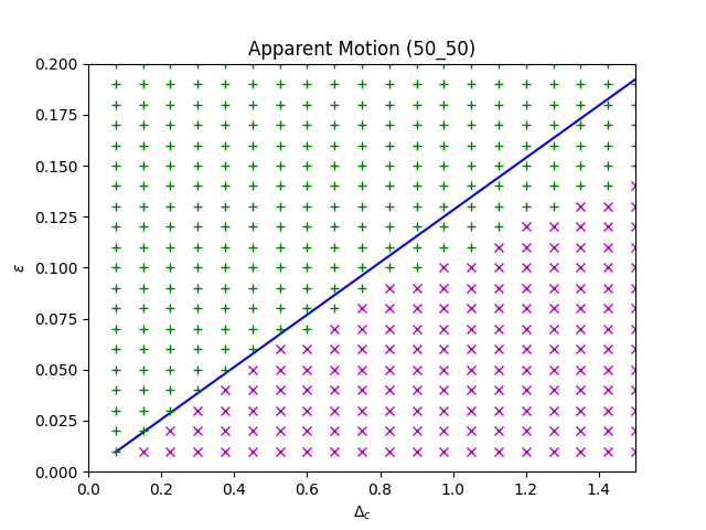
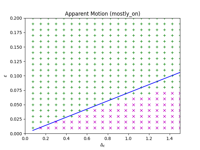
We see that for $y^*$ to exist, we require the denominator of this expression to be positive. That is \begin{align*} -\frac{\Delta_c T}{c\tau_u} &\gt -\frac{\varepsilon T_\text{on}}{D} \\ \Delta_c &\lt \varepsilon \frac{T_\text{on}}{T}\frac{c\tau_u}{D} \end{align*} and we have a condition on entrainment.
Furthermore, this formula is consistent with our intuition. For example, we satisfy this inequality and have a fixed point. If we consider continuously reducing the magnitude $\varepsilon \searrow \Delta_c \frac{T D}{T_\text{on}c\tau_u}$, we find that the denominator in the argument to the logarithm remains positive and tends toward zero, thus $y^* \to -\infty$. When $\varepsilon$ reaches this value or goes below it, the inequality no longer holds and $y^*$ is undefined. In particular, $\varepsilon = 0$ will fail to entrain if $\Delta_c \lt 0$, as we expect.
As another example, consider taking $T_\text{on} \to 0$ while keeping $T$ fixed (so $T_\text{off} = T - T_\text{on}$). We find that the right hand side of this inequality goes to zero and eventually entrainment breaks. This makes sense, as the portion of the period where the stimulus is on is vanishing and thus providing less acceleration each period.
Lastly, we note that this fixed point iteration is stable so long as the fixed point exists. We check \begin{align*} F'(x) &= -\frac{1}{r} \frac{1}{\frac{b}{a} + \left(e^{-rx} - \frac{b}{a}\right)e^{-arT_\text{on}}} (-r)e^{-rx}e^{-arT_\text{on}} \\ &= \frac{e^{-rx}e^{-arT_\text{on}}}{\frac{b}{a} + \left(e^{-rx} - \frac{b}{a}\right)e^{-arT_\text{on}}} \\ &= \frac{e^{-rx}e^{-arT_\text{on}}}{e^{-rx}e^{-arT_\text{on}} + \frac{b}{a} (1-e^{-arT_\text{on}})} \\ &= \frac{1}{1 + \frac{b}{a} \frac{1-e^{-arT_\text{on}}}{e^{-rx}e^{-arT_\text{on}}}} \\ F'(y^*) &= \frac{1}{1 + \frac{b}{a} \frac{1-e^{-arT_\text{on}}}{e^{-ry^*}e^{-arT_\text{on}}}} \\ &= \frac{1}{1 + \frac{b}{a} \frac{1-e^{-arT_\text{on}}}{\frac{b}{a} \frac{1-e^{-arT_\text{on}}}{e^{-rK} - e^{-arT_\text{on}}} e^{-arT_\text{on}}}} \\ &= \frac{1}{1 + \frac{e^{-rK} - e^{-arT_\text{on}}}{e^{-arT_\text{on}}}} \\ &= \frac{e^{-arT_\text{on}}}{e^{-arT_\text{on}} + e^{-rK} - e^{-arT_\text{on}} }\\ &= e^{rK - arT_\text{on}} \end{align*} then \begin{align*} |F'(y^*)| \lt 1 &\iff rK \lt arT_\text{on} \\ & \iff \Delta_c \lt \varepsilon \frac{T_\text{on}}{T}\frac{c\tau_u}{D} \end{align*} and we have that the fixed point iteration is stable provided $y^*$ exists.
Consistency with finite width
We can improve this bound by incorporating the consistency condition $y^* \gt \hat{y} - \Delta_y$. That is, we require the fixed point not to fall behind the stimulus entirely. We proceed \begin{align*} \Delta_y &\gt \frac{1}{r} \log\left[ \frac{b_1}{a} \frac{e^{T_{\text{on}}/\tau_u} - e^{-\varepsilon T_\text{on} / D}}{e^{-\Delta_c T r} - e^{-\varepsilon T_\text{on} / D}} \right] \\ e^{r \Delta_y} &\gt \frac{b_1}{a} \frac{e^{T_{\text{on}}/\tau_u} - e^{-\varepsilon T_\text{on} / D}}{e^{-\Delta_c T r} - e^{-\varepsilon T_\text{on} / D}} \\ e^{r \Delta_y} \left(e^{-\Delta_c T r} - e^{-\varepsilon T_\text{on} / D}\right) &\gt \frac{b_1}{a} \left(e^{T_{\text{on}}/\tau_u} - e^{-\varepsilon T_\text{on} / D}\right) \\ e^{-\Delta_c T r} &\gt \frac{b_1}{a} e^{-r\Delta_y} \left(e^{T_{\text{on}}/\tau_u} - e^{-\varepsilon T_\text{on} / D}\right) + e^{-\varepsilon T_\text{on} / D} \\ \Delta_c &\lt - \frac{c\tau_u}{T} \log\left[ \frac{b_1}{a} e^{-r\Delta_y} \left(e^{T_{\text{on}}/\tau_u} - e^{-\varepsilon T_\text{on} / D}\right) + e^{-\varepsilon T_\text{on} / D} \right] \\ \end{align*} Observe that if we were to take $\Delta_y \to \infty$ then $e^{-r\Delta_y} \to 0$ and this reduces to the same condition as before.
Simulation
We compare our asymptotic approximation to a grid of pulse magnitudes and relative pulse speeds for several configurations of $T_\text{on}$ and $T_\text{off}$. We name these scenarios 50 50 ($T_\text{on}=0.5, T_\text{off}=0.5$), mostly on ($T_\text{on}=0.5, T_\text{off}=0.05$), and mostly off ($T_\text{on}=0.05, T_\text{off}=0.5$). Other parameters are chosen as our standard pulse experiment $\tau_u = 1, \tau_q = 20, \theta=0.2, \beta = 5$.