April 24th, 2023
We apply our asymptotic wave response approximation to a moving localized stimulus. We determine that the asymptotic formulation cannot differentiate between entrainment and non-entrainment and thus a new formulation is required.
Entrainment Simulations
For some moving localized stimuli, we observe a phenomenon called entrainment: the speed of the traveling wave adjusts to match the speed of the stimulus. We say that the wave has entrained to the stimulus. We are interested in entrainment as a possible control mechanism. Figure 1 shows an example of a traveling pulse solution accelerating (and changing profile) to match the speed of a moving Gaussian stimulus. As the stimulus overtakes the front of the pulse, we see the pulse accelerates to match the stimulus speed and a new steady-state in the traveling-stimulus coordinate frame is achieved.
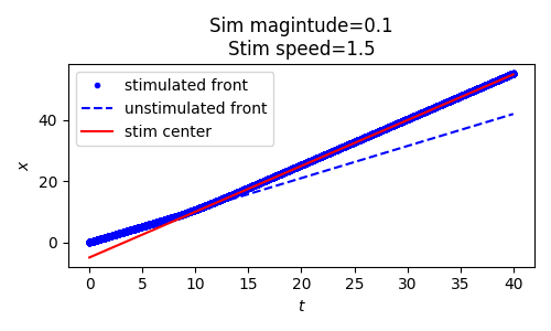
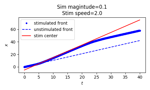
Not all localized moving stimuli achieve entrainment. For example, if a weak stimulus is moving to quickly, it will outpace a traveling pulse solution before it can accelerate the traveling pulse to match its speed. Figure 2 below shows two simulations (again with a moving Gaussian stimulus) that vary in their speed and thus achieve entrainment (left) or fail to achieve entrainment (right).
Weak moving Gaussian stimuli can be characterized by their magnitude (specifically their maximum value) and their speed. Figure 3 roughly partitions this domain into regions of entrainment and regions of non-entrainment using numerical simulation. We see that strong slow stimuli entrain, while weak fast stimuli fail to entrain.

The objective of this report is to determine if our asymptotic wave-response approximation can be used to predict entrainment of stimuli. Before we address this, we first make a few observations about entrainment.
Firstly, our wave response predicts no way to meaningfully slow our traveling pulses, and similarly we expect that our pulses cannot entrain to stimuli slower than the natural speed of the traveling pulses. This is somewhat restrictive if we wish to encode a wide range of slow speeds, but can be remedied by choosing appropriate model parameters. In particular, we can artificially change the firing-rate threshold by adding a constant external stimulus to achieve a wide range of wave speeds. This is straightforward to do analytically and has been observed in vitro (citation needed).
We also note that if a stimulus is strong enough to actually generate traveling wave solutions then it may not be appropriate to say that the traveling pulse entrains to the stimulus. We avoid resolving this issue by only considering weak stimuli.
Lastly, and keeping the previous limitation in mind, we require a formal definition of entrainment if we are to address the question analytically. To that end we define entrainment as follows: for a traveling pulse with natural speed $c$, and a moving localized stimulus with constant speed $d = c + \Delta_c$ for $\Delta_c > 0$, we say that the pulse entrains to the stimulus if the fore threshold crossing of the pulse is $o(d \cdot t + K)$ for some constant $K \in \RR$.
Asymptotic Wave Response
While the numerical simulations above use moving Gaussian stimuli, we will instead use moving square pulses as they are more amenable to analytic calculation. For a direct comparison, we ought to redo the simulations above using a moving square stimulus, be we expect the results to be similar and thus will forgo a direct comparison for the time being.
In general, a moving stimulus can be expressed $$ I_u(\xi, t) = g(\xi - \Delta_c \cdot t) $$ in the traveling wave coordinate frame, where $\Delta_c$ is the difference between the stimulus speed and the natural wave speed and $g$ is a pulse profile that is constant with respect to time. In particular, we will use the square pulse $$ I_u(\xi, t) = \varepsilon I_{(0, 1)}(\xi - \Delta_c \cdot t) $$ where $$ I_A(\xi) = \begin{cases} 1, & \xi \in A \\ 0, & \text{else} \end{cases} $$ is an indicator function.
Applying our asymptotic approximation we find $$\begin{align*} \nu(t) \propto& \int_0^t \int_\mathbb{R} v_1(\xi) \cdot I_u(\xi, \tau) \ d\xi d\tau \\ &= \int_0^t \int_\mathbb{R} H(\xi)e^{-\xi/c\mu} \varepsilon I_{(0, 1)}(\xi - \Delta_c \cdot \tau) \ d\xi d\tau \\ &= \varepsilon \int_0^t \int_\mathbb{R} e^{-\xi/c\mu} I_{(\Delta_c \tau, \Delta_c \tau + 1)}(\xi) \ d\xi d\tau \\ &= \varepsilon \int_0^t \int_{\Delta_c \tau}^{\Delta_c \tau + 1} e^{-\xi/c\mu} \ d\xi d\tau \\ &= \varepsilon \int_0^t c\mu (e^{(-\Delta_c \tau)/c\mu} - e^{-(\Delta_c \tau + 1)/c\mu} \ d\tau \\ &= c\mu \big( 1 - e^{-1/c\mu} \big) \varepsilon \int_0^t e^{-\Delta_c \tau /c\mu} \ d\tau \\ &= \frac{c^2\mu^2 \big( 1 - e^{-1/c\mu} \big)}{ \Delta_c} \varepsilon \big( 1 - e^{-\Delta_c t /c\mu} \big). \end{align*}$$
This predicts a finite wave response in the $t \to \infty$ limit which is inconsistent with entrainment. At best, we expect this to be a reasonable approximation when the stimulus parameters ($\Delta_c$ and $\varepsilon$) place us far away from the domain of entrainment.
We note that for small $t$, we can Taylor expand this approximation $$\begin{align*} \nu(t) \propto c \mu (1 - e^{-1/c\mu}) \varepsilon t + \mathcal{O}(\Delta_c^2) \end{align*}$$ and see that up to leading order, the response has speed $$ \Delta_c^* = c \mu (1 - e^{1/c\mu}) \varepsilon $$ which unfortunately is independent of $\Delta_c$ and does depend on $\varepsilon$ – two properties inconsistent with entrainment.