August 4th, 2021
We highlight the difficulties in finding a stationary bump solution to the adaptive model with a weight-kernel of the form $w(x,y) = M_1 e^{-|x-y|} - M_2 e^{-|x-y|/\sigma}$.
To-Do List Snapshot
- Manuscript
Find template- Outline
- Select figures
- Adjoint method: explore different weight kernels.
- Derive interface equations.
- Convergent Solver (low priorety)
- Stability Analysis (low priorety)
- Wave-train Analysis
- Find periodic solutions.
- Compare frequency and pulse width to non-periodic solutions.
- Reading
- Coombes 2004.
- Folias & Bressloff 2005.
- Faye & Kilpatrick 2018.
Stationary Bumps
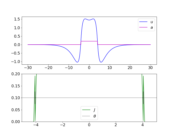
This week we explored the adaptive model, but with weight-kernel which can be described as the difference of exponential functions: $$\begin{align*} \mu u_t &= -u + \int_\RR \big( M_1 e^{-|x-y|} - M_2 e^{-|x-y|/\sigma}\big) H(u(y) - a(y) - \theta) \ dy \\ \alpha a_t &= -a + \gamma H(u - a - \theta). \end{align*}$$ Non-adaptive models that use this weight-kernel are known to exhibit stationary bump solutions. Numerical simulations suggest something similar happens in the adaptive case, as seen in the simulation below.
The simulation suggests that there may be some stationary bump solution around which this solution is oscillating. However, we believe that such a solution does not exist.
Non-existence of stationary bumps
For a stationary solution, we have that $u_t = a_t = 0$, and that the solution is simply a function of $x$ and constant throughout time. We will require that $J = u-a$ crosses threshold exactly twice at WLOG $x= \pm \Delta$ for some half-width $\Delta$, and that $J$ is super-threshold only between these two points.
Our system then reduces significantly $$\begin{align*} u &= \int_{-\Delta}^\Delta M_1 e^{-|x-y|} - M_2 e^{-|x-y|/\sigma} \ dy \\ a &= \gamma \big( H(x + \Delta) - H(x - \Delta) \big) \end{align*}$$ and in fact is decoupled, except by the value of $\Delta$. From this formulation it is apparent that $u$ is continuous and that $a$ is discontinuous at $x = \pm \Delta$. This necessarily means that $J$ is also discontinuous at $x = \pm \Delta$, and makes it unclear what boundary conditions to apply.
The simulation in Figure 1 was initialized by this analytic solution, choosing $\Delta$ such that $$ u(\pm \Delta) = \theta + \tfrac{1}{2} \gamma = \theta + \frac{\lim\limits_{\xi \to \pm \Delta^+} a(\xi) + \lim\limits_{\xi \to \pm \Delta^-} a(\xi)}{2}. $$ We plot this solution below, and see that it violates our assumption of $J = u-a$ having exactly two threshold crossings.