June 24th, 2021
We have begun using a semi-analytic implementation for simulations. The reduced computational complexity allows for efficient higher resolution simulations.
To-Do List Snapshot
- Investigate wave-response function.
- Convert to a semi-analytic implementation.
Spatially homogeneous pulse.- Spatially homogeneous, temporally finite.
- Local pulses.
- Wave-train Analysis
- Search the literature.
- Find periodic solutions.
- Compare frequency to a pair of pulses.
- Reading
- Coombes 2004.
- Folias & Bressloff 2005.
- Faye & Kilpatrick 2018.
Semi-analytic implementation
Previously we proposed to switch to a semi-analytic implementation where the convolution is integrated analytically, based on numerically approximated threshold-crossings. In particular, we hoped that with some combination of cusp-detection and left/right interpolation we could achieve a higher order of accuracy.
This has proven more difficult than anticipated. In particular, identifying threshold crossings to first order is non-trivial. In theory, our solutions should be smooth except for a few (time-dependent) positions in space, and the threshold-crossings should be clear. However, oscillations relative to the pulse-speed in the approximations of the threshold crossings are immediately propagated to all points in the solution, due to the convolution.
The result is that if the time-discretization is large relative to the spatial discretization, then the solution vector will exhibit spurious threshold crossings. Our current implementation throws an assertion error when it detects more than two threshold-crossings. This limitation is somewhat reminiscent of the CFL condition for numerical solutions to hyperbolic PDEs, though we suspect the connection is superficial. For now we will restrict our focus to simulation resolutions in which the first-order threshold-crossing approximations are unambiguous.
We have hypothesized that using polynomial interpolation to approximate the threshold-crossings and a high-order time integration scheme would not achieve high-order accuracy due to non-smoothness of the firing-rate function. Ultimately, we are not concerned with the order of accuracy, but we require the simulations be accurate enough and fast enough. Figure 1 shows measurements of the speed of simulated traveling pulses. They all have spatial resolution $h = 2^{-7}$ and temporal resolution $k= 2^{-8}$. They differ in the time-integration scheme used, and the order of polynomial interpolation used in the threshold-crossing process.

While this is not a convergence study (and thus does not verify the order of accuracy of these simulations) we can clearly see that choosing the higher order method results in higher accuracy for these simulations. Additionally, the semi-analytic method has complexity $O(n)$ per time-step regardless of the degree of polynomial interpolation, which is an improvement on the $O(n^2)$ quadrature used previously. We believe that it may be enough to simply use this implementation but increase the resolution.
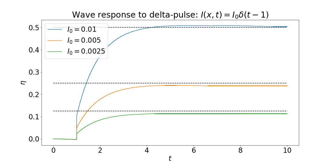
As a proof of concept, in Figure 2, we successfully reproduced the wave-response function results from last week, but this time adjusting the front measurements using the analytic pulse speed. The results match Figures 1 and 3 of the previous report.
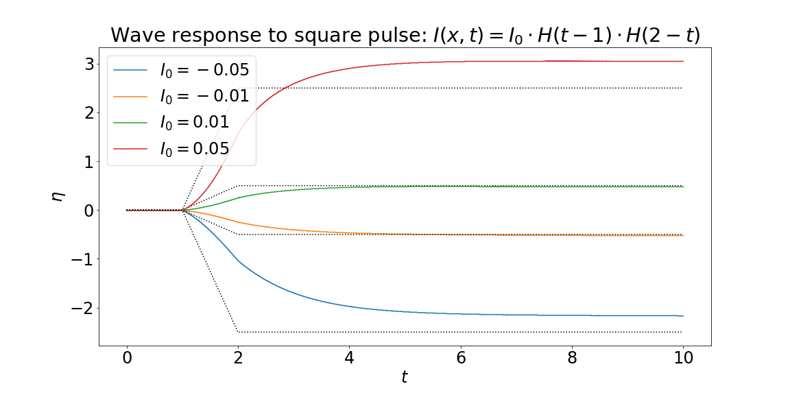
Similarly, Figure 3 shows our simulated wave-response to the stimulus $I(x,t) = I_0 H(t-1) H(2-t)$ (the square-pulse).