Wave response theory for neural representations of apparent motion
Sage Shaw - Oct 20th, 2023
Kilpatrick Lab at University of Colorado Boulder
The Kilpatrick Lab
Prof. Zack Kilpatrick

Dr. Tahra Eissa

Heather Cihack
Sage Shaw
Outline
- Neural field model
- Traveling wave solutions
- The wave response function
- Entrainment
- Apparent Motion Entrainment
- Future Work
Neural Field Model
Biological Neural Networks
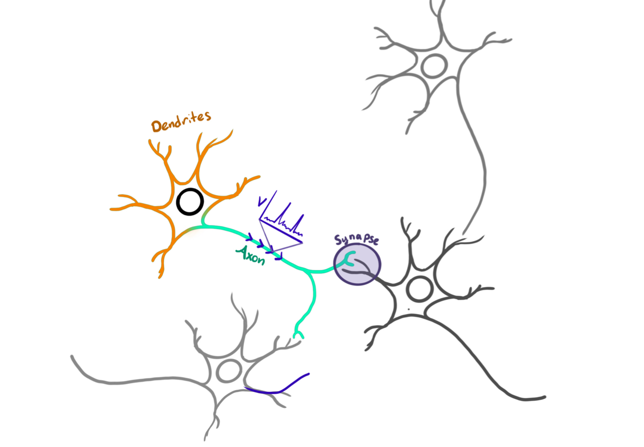
Image courtesy of Heather Cihak.
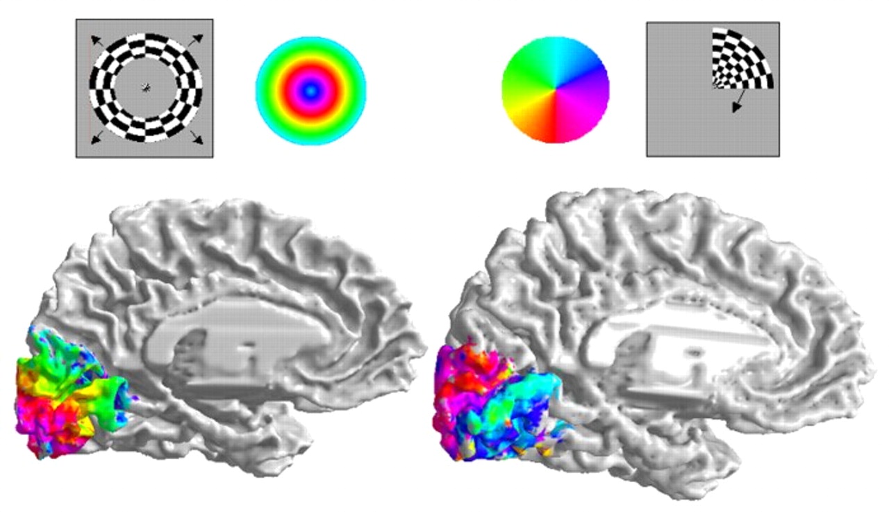
Retinotopic Map
- Primary visual area (V1)
- Sensory areas have spatially organized topologies
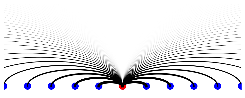
Neural Field Models
- Organize neural populations on a line
- Connectivity is determined by distance
- Extend to a continuum limit
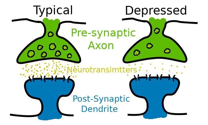
Synaptic Depression
Rapid firing depletes pre-synaptic resources.
Model
\begin{align*} \tau_u \frac{\partial}{\partial t}\underbrace{u(x,t)}_{\text{Activity}} &= -u + \underbrace{\overbrace{w}^{\substack{\text{network}\\\text{connectivity}\\\text{kernel}}} \ast \big( q f[u] \big)}_{\substack{\text{network}\\\text{stimulation}}} \\ \tau_q \frac{\partial}{\partial t}\underbrace{q(x,t)}_{\substack{\text{Synaptic}\\\text{Efficacy}}} &= 1 - q - \underbrace{\beta}_{\substack{\text{rate of}\\\text{depletion}}} q \underbrace{f(u)}_{\substack{\text{firing-rate}\\\text{function}}} \end{align*}
Model
- $f[u] = H(u - \theta)$ - All or nothing firing-rate function.
- $w(|x-y|) = \frac{1}{2}e^{-|x-y|}$ - network connectivity kernel
- $\gamma = \frac{1}{1+\beta} \in (0, 1]$
1D Neural Fields
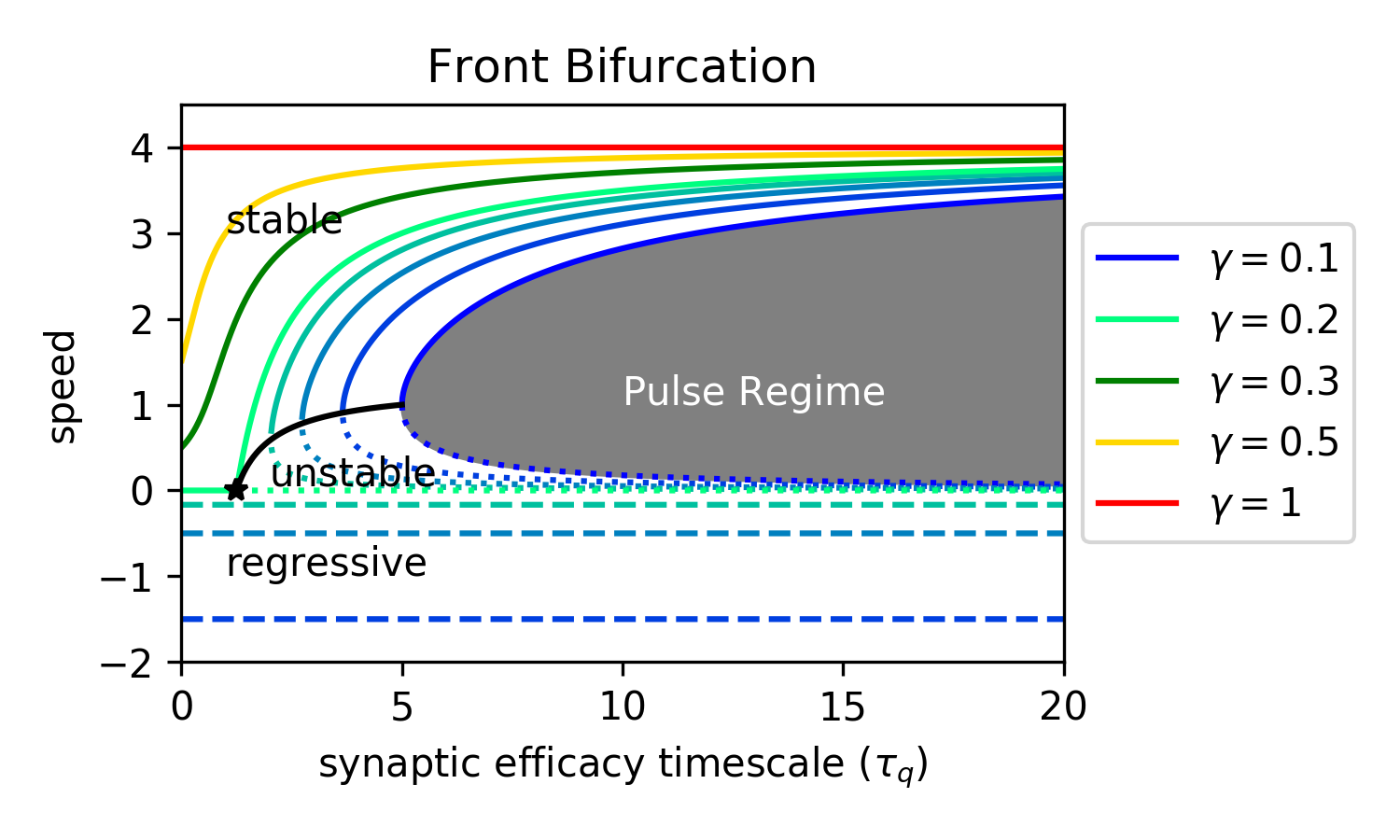
- Progressive fronts
- Regressive fronts
- Pulses
Wave response
Correcting Position
- Position encoded as a pulse
- Must be corrected
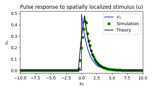
Spatially localized perturbation
Asymptotic Approximation
add stimulus terms $$ \begin{align*} \tau_u u_t &= -u + w * (q f[u]) + \varepsilon I_u(x, t) \label{eqn:forced_u} \\ \tau_q q_t &= 1 - q - \beta q f[u] + \varepsilon I_q(x, t) \label{eqn:forced_q} \end{align*} $$substitute with the expansion $$ \begin{align*} u(\xi, t) &= U\big( \xi - \varepsilon \nu(t) \big) + \varepsilon \phi\big(\xi - \varepsilon \nu(t), t\big) + \mathcal{O}(\varepsilon^2) \\ q(\xi, t) &= Q\big( \xi - \varepsilon \nu(t) \big) + \varepsilon \psi\big(\xi - \varepsilon \nu(t), t\big) + \mathcal{O}(\varepsilon^2) \end{align*} $$
Collect the $\mathcal{O}(\varepsilon)$ terms
$$\begin{align*} \underbrace{\begin{bmatrix}\tau_u & 0 \\ 0 & \tau_q\end{bmatrix}}_{T} \begin{bmatrix}\phi \\ \psi \end{bmatrix}_t + \mathcal{L}\begin{bmatrix}\phi \\ \psi \end{bmatrix} &= \begin{bmatrix} I_u + \tau_u U' \nu' \\ I_q + \tau_q Q' \nu ' \end{bmatrix} \end{align*}$$ $$ \mathcal{L}(\vec{v}) = \vec{v} - cT \vec{v} + \begin{bmatrix} -w Q f'(U) * \cdot & -w f(U) * \cdot \\ \beta Q f'(U) & \beta f(U) \end{bmatrix} \vec{v} $$Bounded solutions exist if the inhomogeneity is orthogonal to $\mathcal{N}\{\mathcal{L^*}\}$. For $(v_1, v_2) \in \mathcal{N}\{\mathcal{L^*}\}$ $$\begin{align*} -c \tau_u v_1' &= v_1 - Qf'(U) \int w(y,\xi) v_1(y) \ dy + \beta Qf'(U) v_2 \\ -c \tau_q v_2' &= v_2 - f(U) \int w(y, \xi) v_1(y) \ dy + \beta f(U) v_2. \end{align*}$$
Wave response function
$$ \frac{\partial}{\partial t}\nu = \frac{ \langle v_1 ,I_u(\xi + \color{blue}{\varepsilon \nu}, t)\rangle + \langle v_2, I_q(\xi +\color{blue}{\varepsilon \nu}, t)\rangle }{\underbrace{-\tau_u \langle v_1, U' \rangle - \tau_q \langle v_2, Q' \rangle}_{K}} $$Spatially localized perturbation
Entrainment
Tracking a moving stimulus

Tracking a moving stimulus
Entraining to a moving stimulus
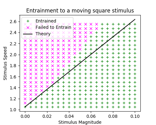
Asymptotic threshold
$$ \Delta_c \lt \varepsilon \frac{c\tau_u}{K}$$
Asymptotic Entrainment Threshold
$$ \Delta_c < \varepsilon \frac{c\tau_u}{K} \frac{T_\text{on}}{T} $$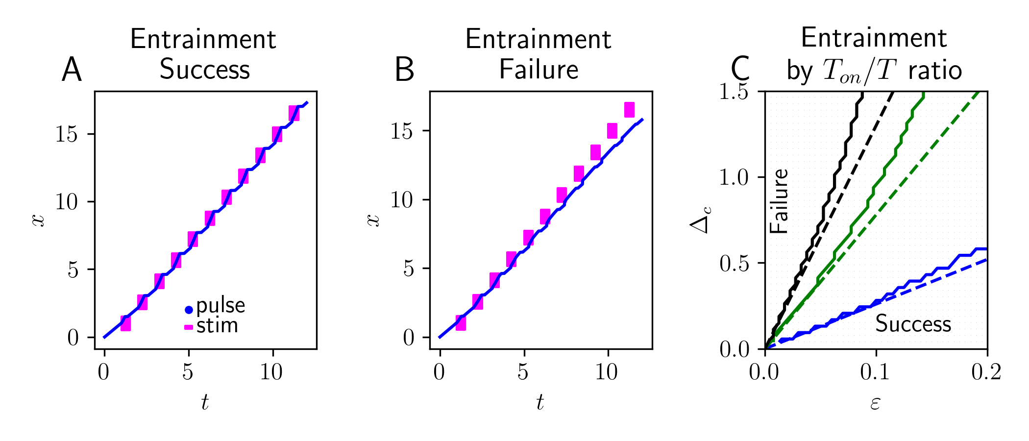
Future work
Spreading Depression
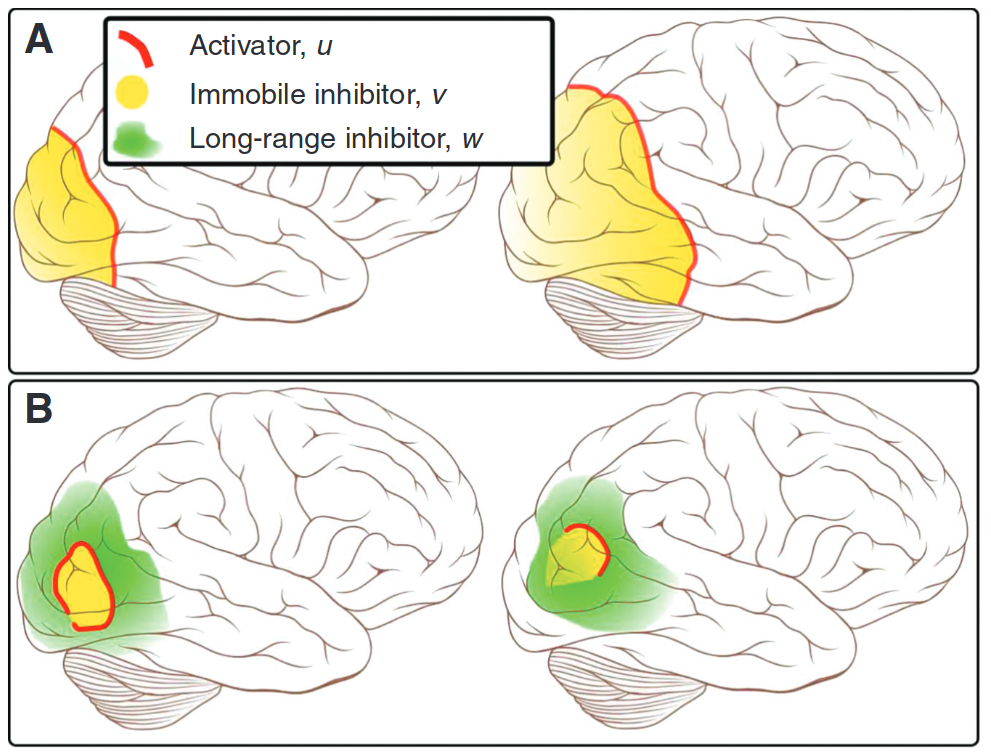
Zandt, Haken, van Putten, and Markus (2015)
Retinotopic Map
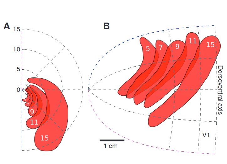
Zandt, Haken, van Putten, and Markus (2015)
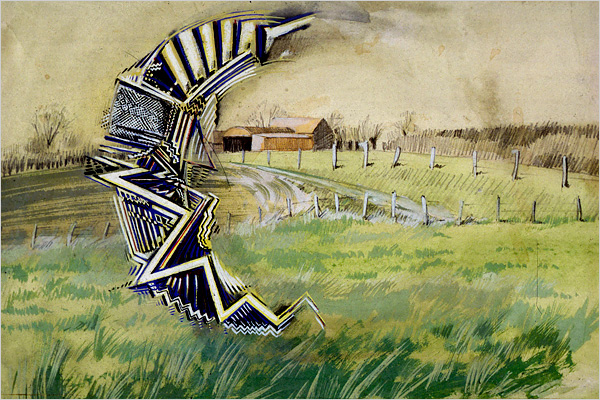
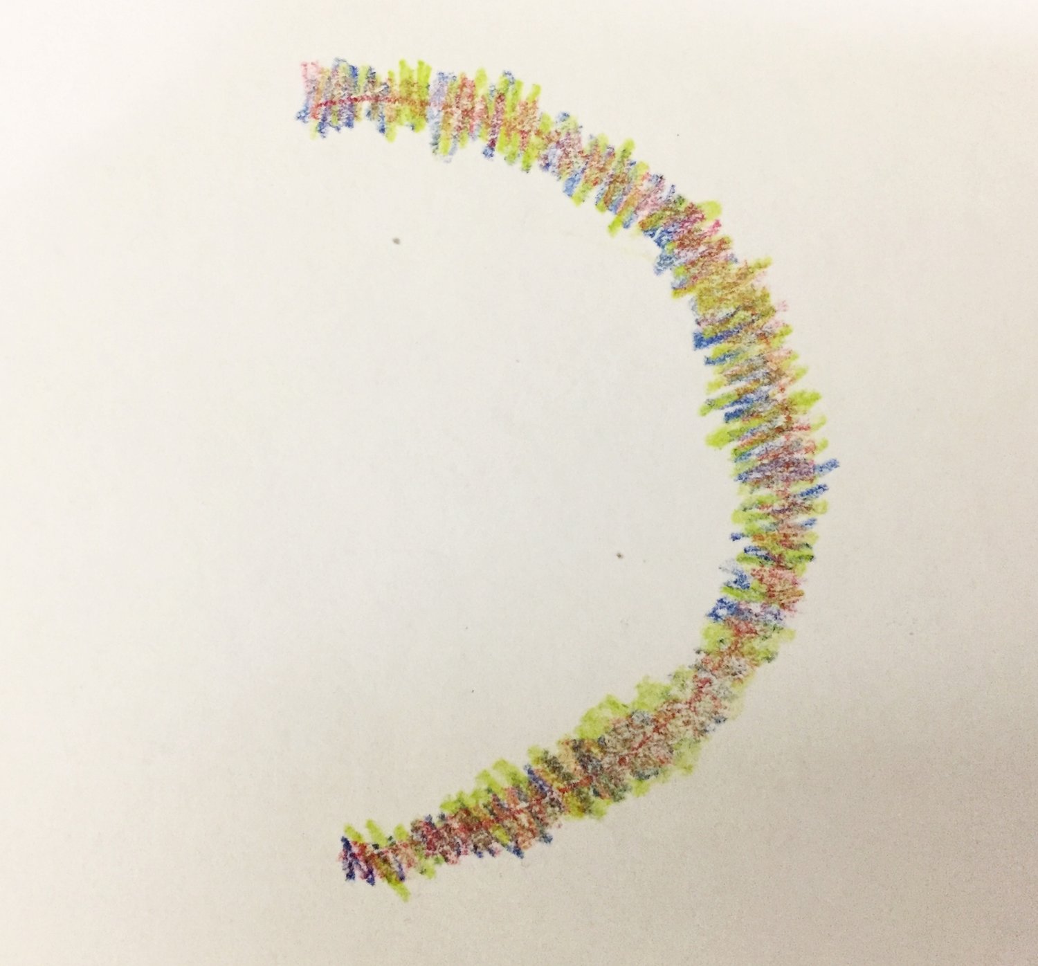
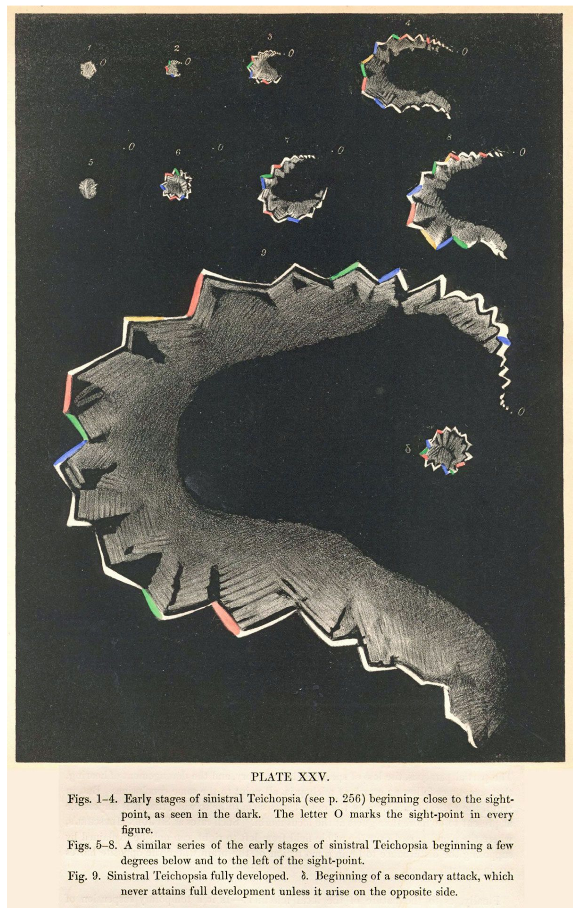
Scintillating Scotoma
Reaction Diffusion Model
$$\begin{align*} u_t &= \underbrace{u - \frac{1}{3}u^3}_{\text{excitable}} - \underbrace{v}_{\text{recovery}} + \underbrace{D\nabla^2 u}_{\text{Diffusion}} \\ \frac{1}{\varepsilon} v_t &= u + \beta + \underbrace{K\int H(u) d \Omega}_{\substack{\text{neurovascular}\\\text{feedback}}} \end{align*}$$
Reaction Diffusion on surfaces
$$\begin{align*} u_t &= 3u - u^3 - v + D \Delta_{\mathcal{M}}u \\ \frac{1}{\varepsilon} v_t &= u + \beta + K \int_{\mathcal{M}} H(u) \ d \mu_{\mathcal{M}} \end{align*}$$
- Surface operators: $\Delta_{\mathcal{M}}, \int_{\mathcal{M}} \cdot d \mu_{\mathcal{M}}$
- Affects speed and stability of waves
Coupled neural field and diffusion equation
$$\begin{align*} v_t &= -v + w \ast s_p(v, k) + g_v \\ k_t &= \delta k_{xx} + g_k(s, s_p, a, b) + I \end{align*}$$- Neural field model
- Coupled potassium concentration
- Models both ignition and propagation of CSD
A Turing Reaction Diffusion System using RBFs
$$\begin{align*} u_t &= \delta_u \Delta_{\mathcal{M}} u + \alpha(1-\tau_1 v^2) + v(1-\tau_2 u)\\ v_t &= \delta_v \Delta_{\mathcal{M}} v + \beta(1-\frac{\alpha\tau_1}{\beta} uv) + u(\gamma-\tau_2 v)\\ \end{align*}$$Thank you
- Manuscript on ArXiv soon!
- Slides and Public Notes: shawsa.github.io
- Code repository: github.com/shawsa/neural-field-synaptic-depression
Auxiliary Slides

Traveling wave solutions
Front solutions
- $\xi = x - ct$
- Active region: $(-\infty, 0)$
- Restrict to $c > 0$
- Linearizes equations
- Decouples $q$ from $u$
- $U(-\infty) = \gamma > \theta$
$$ \theta = \frac{\gamma + c\tau_q\gamma}{2(1+c\tau_q\gamma)(1+c\tau_u)} $$
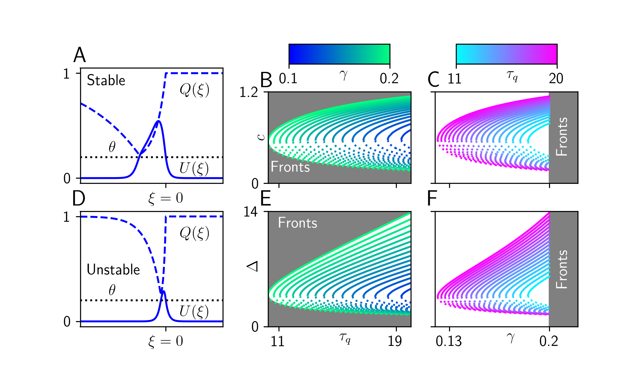
Front Bifurcations
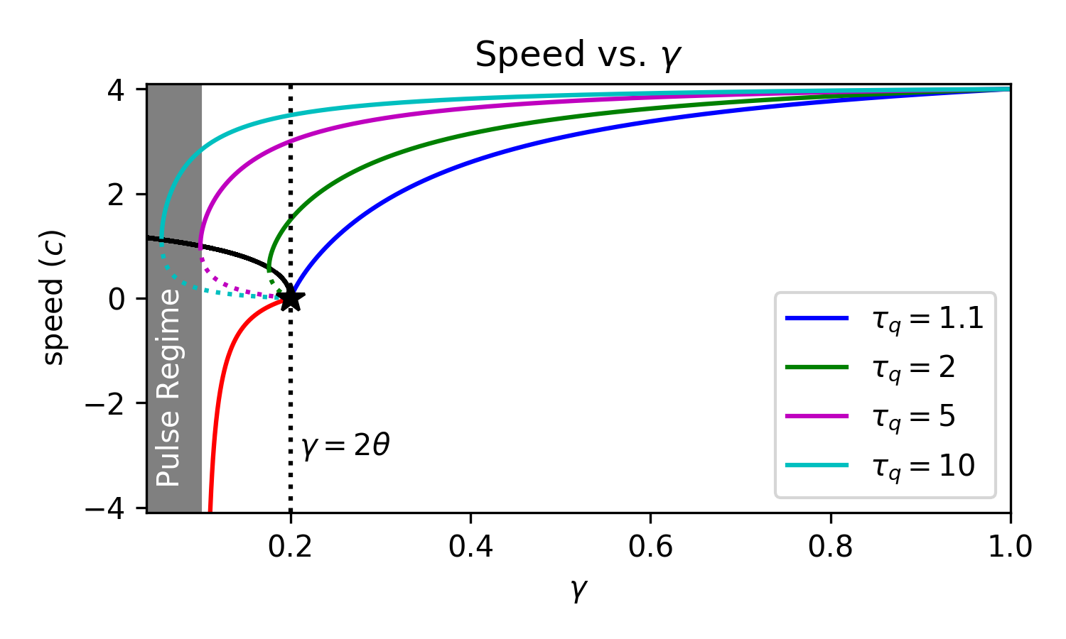
Front Bifurcations
Pulse solutions
- $\xi = x - ct$
- Active region: $(-\Delta, 0)$
- Linearizes equations
- Decouples $q$ from $u$
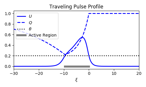
Two consistency equations for $c$ and $\Delta$.
old wave response
$$ \frac{\partial}{\partial t}\nu = \frac{ \langle v_1 ,I_u(\xi, \tau)\rangle + \langle v_2, I_q(\xi, \tau)\rangle }{-\tau_u \langle v_1, U' \rangle - \tau_q \langle v_2, Q' \rangle} $$new wave response
$$ \frac{\partial}{\partial t}\nu = \frac{ \langle v_1 ,I_u(\xi + \color{blue}{\varepsilon \nu}, \tau)\rangle + \langle v_2, I_q(\xi +\color{blue}{\varepsilon \nu}, \tau)\rangle }{\underbrace{-\tau_u \langle v_1, U' \rangle - \tau_q \langle v_2, Q' \rangle}_{K}} $$Pulse Speed and Width