Control of traveling waves in adaptive neural fields
Comprehensive Exam
Sage Shaw - April 4th, 2023
Outline
- Neural field model
- Traveling wave solutions
- The wave response
- Entrainment
- Future work
Neural Field Model
Biological Neural Networks
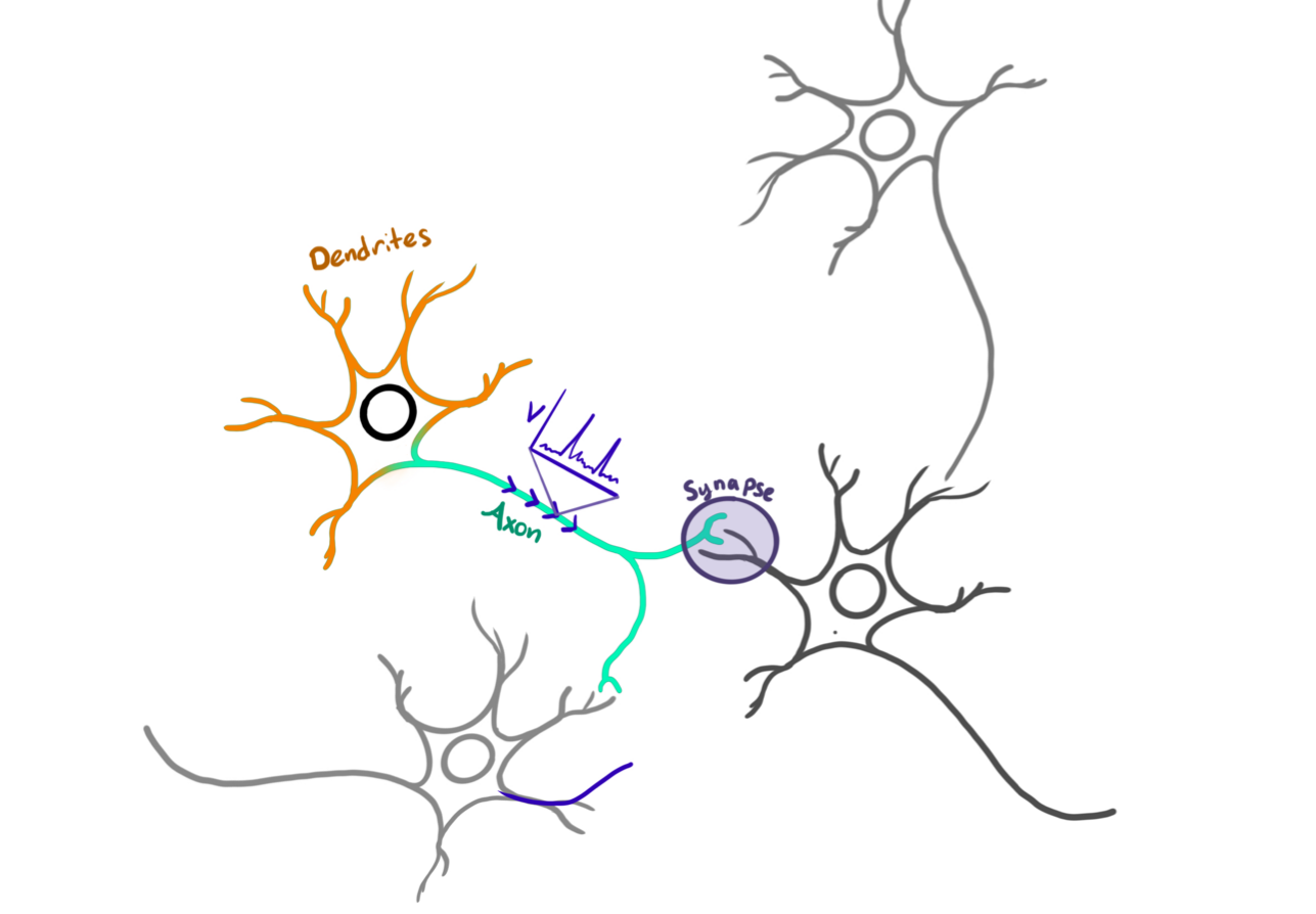
Image courtesy of Heather Cihak.
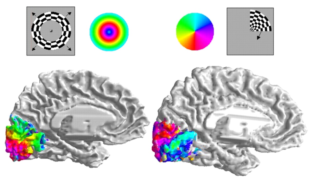
Retinotopic Map
- Primary visual area (V1)
- Sensory areas have spatially organized topologies
Neural Field Models
- Organize neural populations on a line
- Connectivity is determined by distance
- Extend to a continuum limit
1D Neural Fields
- Progressive fronts
- Regressive fronts
- Pulses
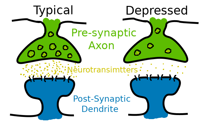
Synaptic Depression
Rapid firing depletes pre-synaptic resources.
Model
\begin{align*} \tau_u \frac{\partial}{\partial t}\underbrace{u(x,t)}_{\text{Activity}} &= -u + \underbrace{\overbrace{w}^{\substack{\text{network}\\\text{connectivity}\\\text{kernel}}} \ast \big( q f[u] \big)}_{\substack{\text{network}\\\text{stimulation}}} \\ \tau_q \frac{\partial}{\partial t}\underbrace{q(x,t)}_{\substack{\text{Synaptic}\\\text{Efficacy}}} &= 1 - q - \underbrace{\beta}_{\substack{\text{rate of}\\\text{depletion}}} q \underbrace{f(u)}_{\substack{\text{firing-rate}\\\text{function}}} \end{align*}
Model
- $f[u] = H(u - \theta)$ - All or nothing firing-rate function.
- $w(|x-y|) = \frac{1}{2}e^{-|x-y|}$ - network connectivity kernel
- $\frac{1}{1+\beta} = \gamma \in (0, 1]$ - Relative timescale of synaptic depletion.
Model
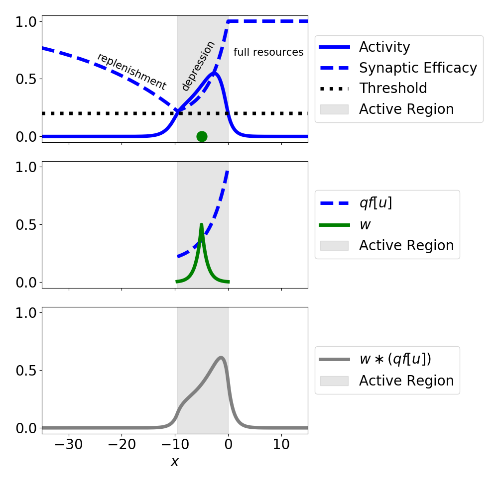
Traveling wave solutions
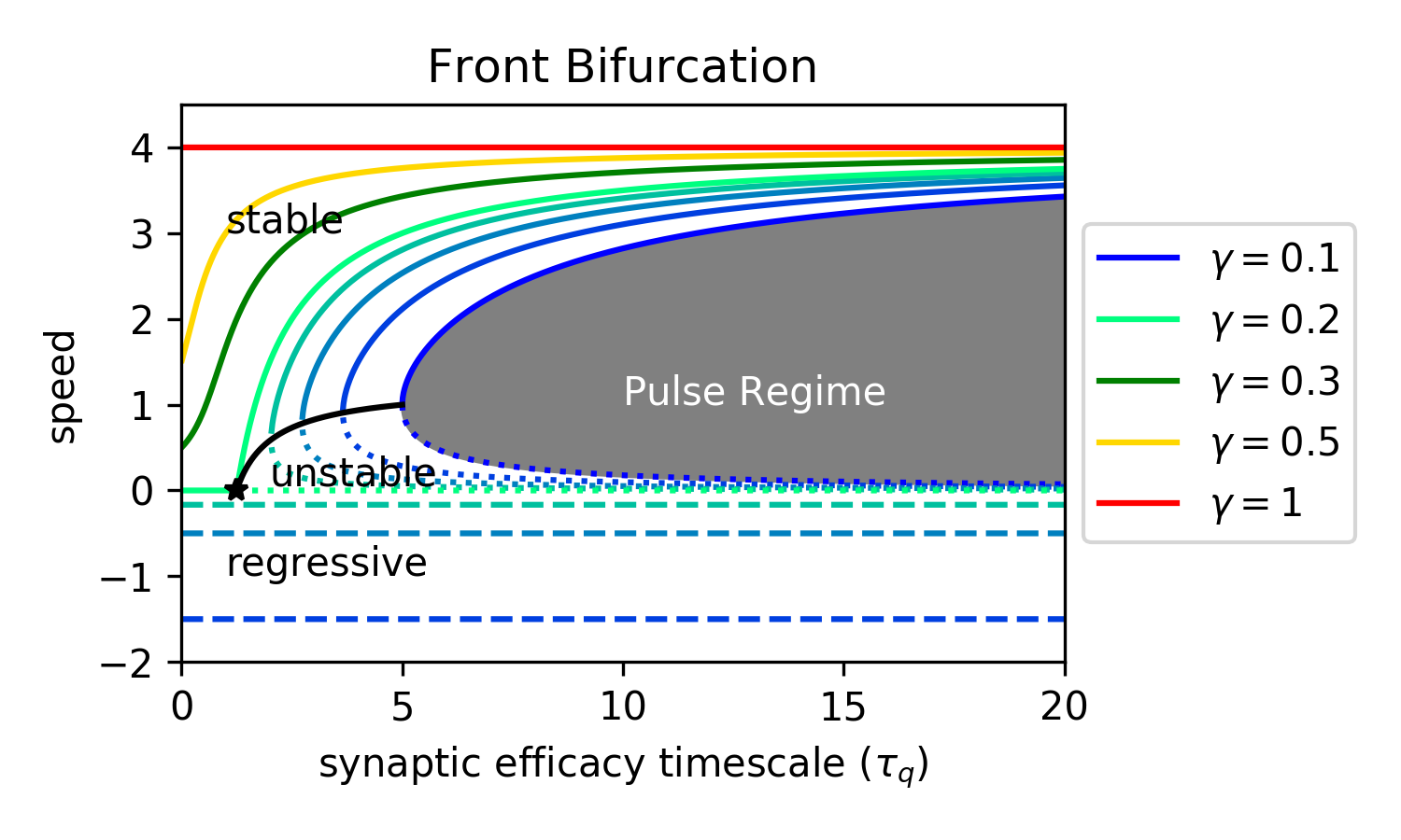
Front solutions
- $\xi = x - ct$
- Active region: $(-\infty, 0)$
- Restrict to $c > 0$
- Linearizes equations
- Decouples $q$ from $u$
- $U(-\infty) = \gamma > \theta$
$$ \theta = \frac{\gamma + c\tau_q\gamma}{2(1+c\tau_q\gamma)(1+c\tau_u)} $$
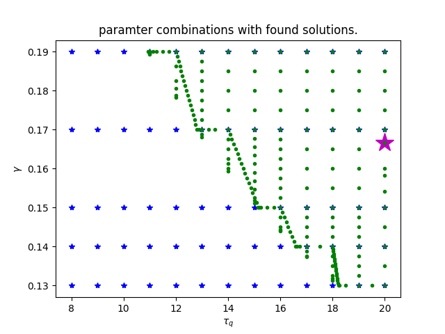
Front Bifurcations
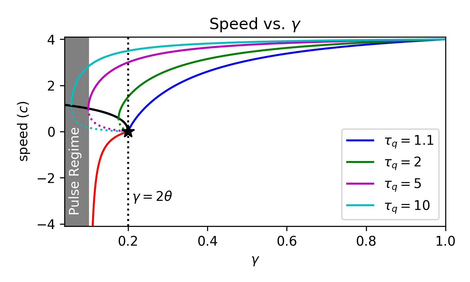
Front Bifurcations
Pulse solutions
- $\xi = x - ct$
- Active region: $(-\Delta, 0)$
- Linearizes equations
- Decouples $q$ from $u$
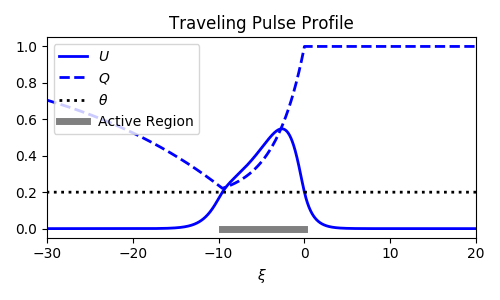
Two consistency equations for $c$ and $\Delta$.
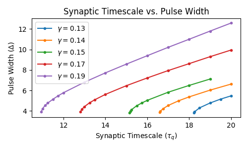
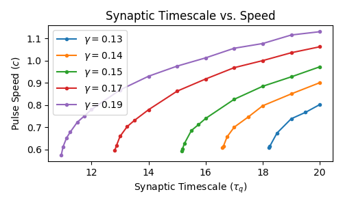
Pulse Speed and Width
Wave response
Correcting Position
- Position encoded as a pulse
- Must be corrected
Spatially homogeneous perturbation
Asymptotic Approximation
add stimulus terms $$ \begin{align*} \tau_u u_t &= -u + w * (q f[u]) + \varepsilon I_u(x, t) \label{eqn:forced_u} \\ \tau_q q_t &= 1 - q - \beta q f[u] + \varepsilon I_q(x, t) \label{eqn:forced_q} \end{align*} $$substitute with the expansion $$ \begin{align*} u(\xi, t) &= U\big( \xi - \varepsilon \nu(t) \big) + \varepsilon \phi + \mathcal{O}(\varepsilon^2) \\ q(\xi, t) &= Q\big( \xi - \varepsilon \nu(t) \big) + \varepsilon \psi + \mathcal{O}(\varepsilon^2) \end{align*} $$
Collect the $\mathcal{O}(\varepsilon)$ terms
$$\begin{align*} \underbrace{\begin{bmatrix}\tau_u & 0 \\ 0 & \tau_q\end{bmatrix}}_{T} \begin{bmatrix}\phi \\ \psi \end{bmatrix}_t + \mathcal{L}\begin{bmatrix}\phi \\ \psi \end{bmatrix} &= \begin{bmatrix} I_u + \tau_u U' \nu' \\ I_q + \tau_q Q' \nu ' \end{bmatrix} \end{align*}$$ $$ \mathcal{L}(\vec{v}) = \vec{v} - cT \vec{v} + \begin{bmatrix} -w Q f'(U) * \cdot & -w f(U) * \cdot \\ \beta Q f'(U) & \beta f(U) \end{bmatrix} \vec{v} $$Bounded solutions exist if the inhomogeneity is orthogonal to $\mathcal{N}\{\mathcal{L^*}\}$. For $(v_1, v_2) \in \mathcal{N}\{\mathcal{L^*}\}$ $$\begin{align*} -c \tau_u v_1' &= v_1 - Qf'(U) \int w(y,\xi) v_1(y) \ dy + \beta Qf'(U) v_2 \\ -c \tau_q v_2' &= v_2 - f(U) \int w(y, \xi) v_1(y) \ dy + \beta f(U) v_2. \end{align*}$$
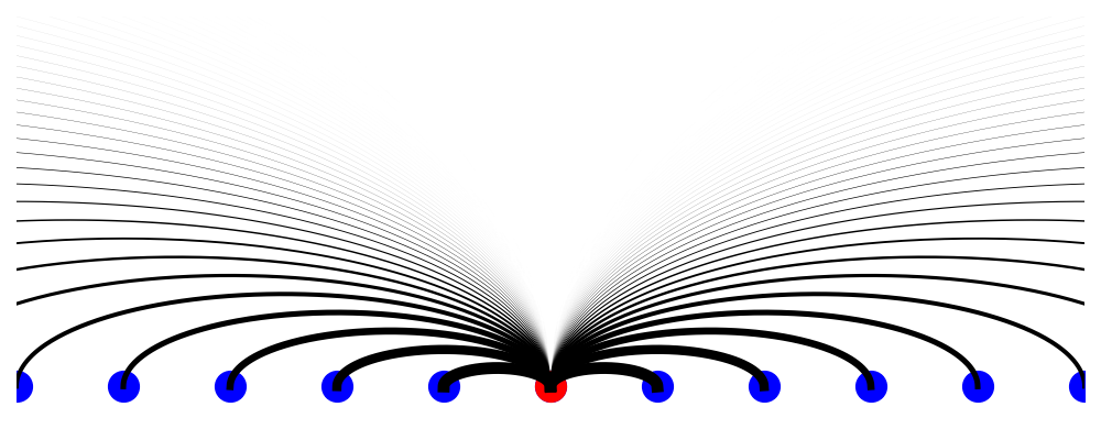
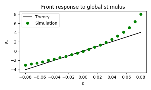
Wave response function
$$ \nu(t) = - \frac{\int_\mathbb{R} v_1 \int_0^t I_u(\xi, \tau) \ d\tau + v_2 \int_0^t I_q(\xi, \tau) \ d\tau \ d\xi}{\int_\mathbb{R} \tau_u U' v_1 + \tau_q Q' v_2 \ d\xi} $$Spatially Homogeneous perturbation
$$ \varepsilon I_u = \varepsilon \delta(t - 1) $$
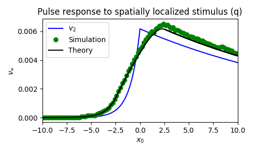
Spatially localized perturbation
Spatially localized perturbation
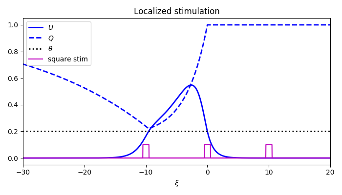
Spatially localized perturbation
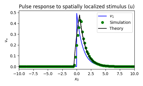
Spatially localized perturbation
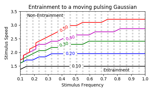
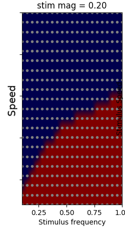
Entrainment
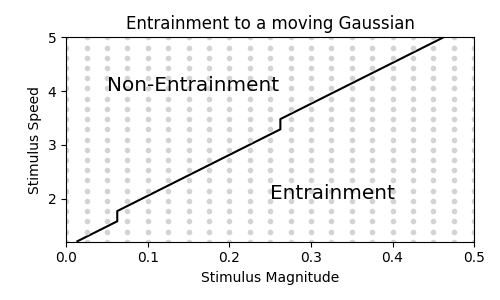
Tracking a moving stimulus

Tracking a moving stimulus
Tracking a moving stimulus
Tracking a flashing stimulus

Tracking a flashing stimulus
Tracking a flashing stimulus
Tracking apparent motion

Tracking apparent motion
Tracking apparent motion
- Preliminary results
- Similar to the moving, flashing stimulus.
Future work
Spreading Depression
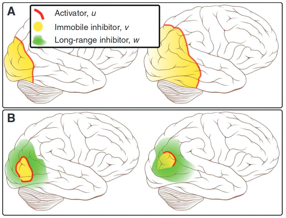
Zandt, Haken, van Putten, and Markus (2015)
Retinotopic Map
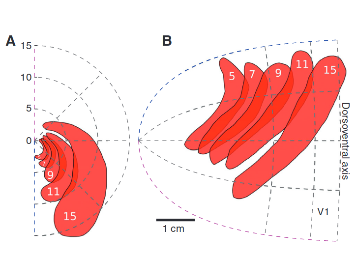
Zandt, Haken, van Putten, and Markus (2015)
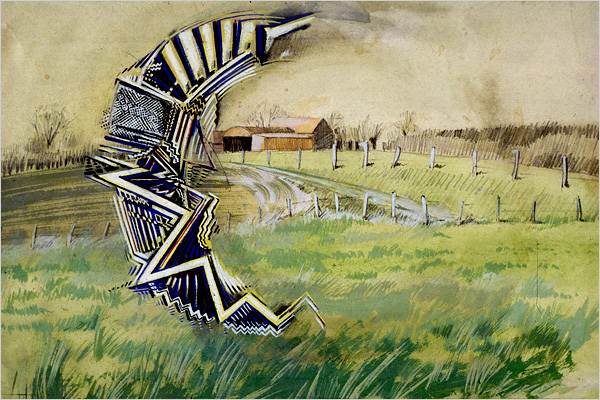
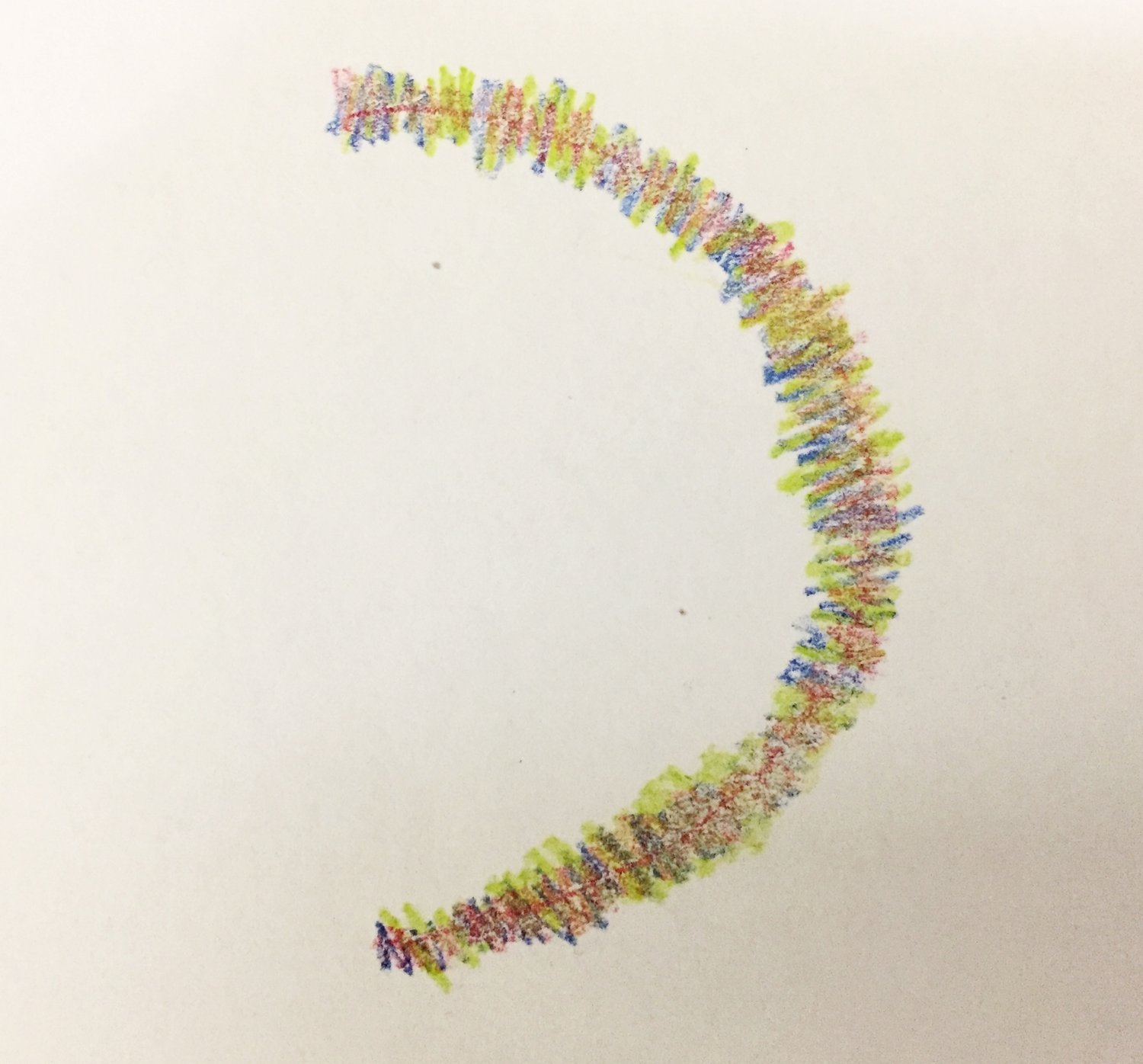
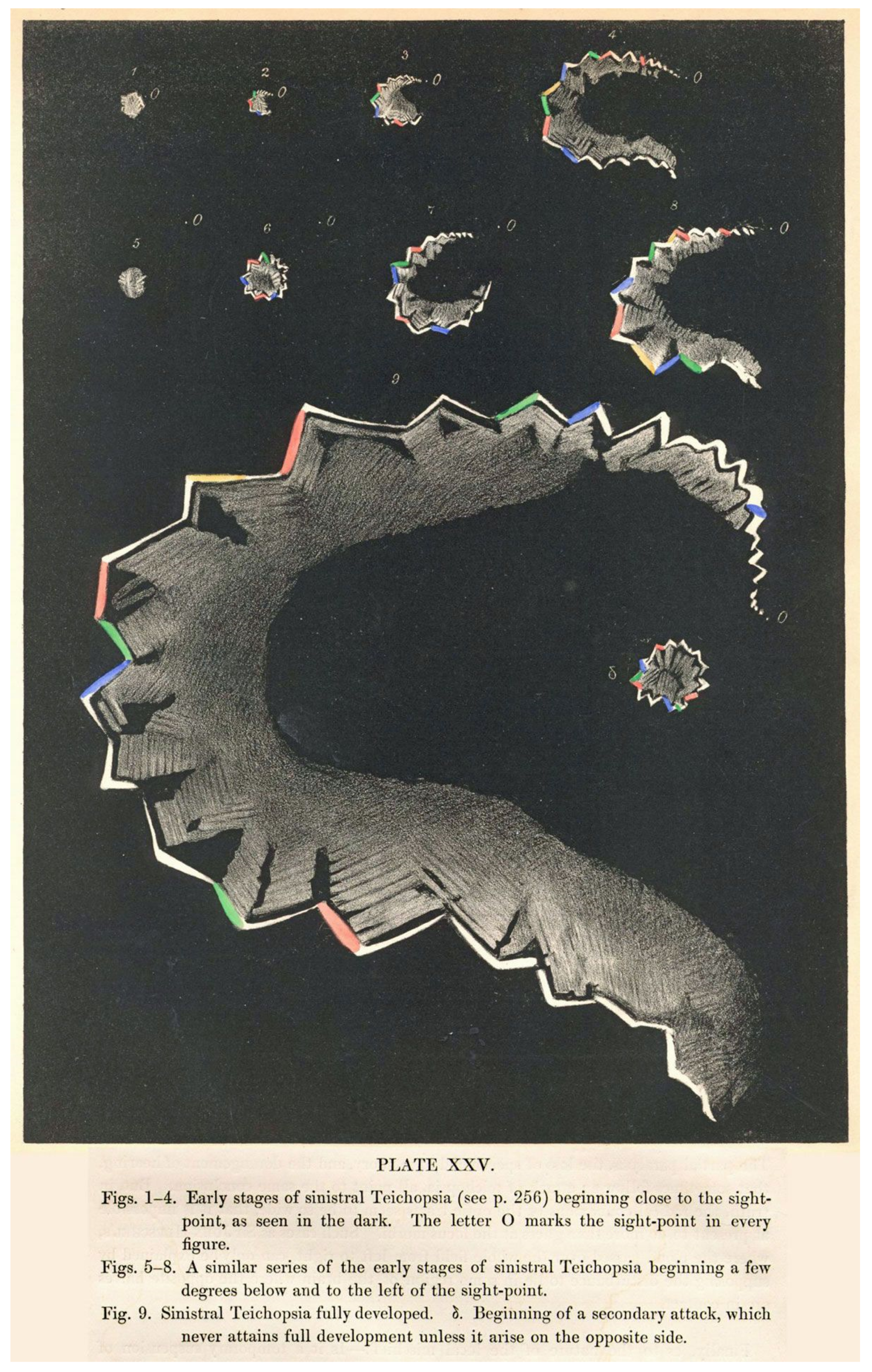
Scintillating Scotoma
Reaction Diffusion Model
$$\begin{align*} u_t &= \underbrace{u - \frac{1}{3}u^3}_{\text{excitable}} - \underbrace{v}_{\text{recovery}} + \underbrace{D\nabla^2 u}_{\text{Diffusion}} \\ \frac{1}{\varepsilon} v_t &= u + \beta + \underbrace{K\int H(u) d \Omega}_{\substack{\text{neurovascular}\\\text{feedback}}} \end{align*}$$
Coupled neural field and diffusion equation
$$\begin{align*} v_t &= -v + w \ast s_p(v, k) + g_v \\ k_t &= \delta k_{xx} + g_k(s, s_p, a, b) + I \end{align*}$$- Neural field model
- Coupled potassium concentration
- Models both ignition and propagation of CSD
Reaction Diffusion on surfaces
$$\begin{align*} u_t &= 3u - u^3 - v + D \Delta_{\mathcal{M}}u \\ \frac{1}{\varepsilon} v_t &= u + \beta + K \int_{\mathcal{M}} H(u) \ d \mu_{\mathcal{M}} \end{align*}$$
- Surface operators: $\Delta_{\mathcal{M}}, \int_{\mathcal{M}} \cdot d \mu_{\mathcal{M}}$
- Affects speed and stability of waves