odeiter

An iterator-based python package for solving systems of differential equations.

Why another ODE solver?

The elephant in the room is scipy.integrate.sovle_ivp. Why would you use odeiter instead? If you want an array of your solution at all time points in a finite interval then solve_ivp is your best solution, but I found myself needing something more flexible. So I made odeiter which takes advantage of Python generators.

Generators decouple the solver code from the looping body. In general, you don't want to simply compute the solution to your system. You want to compute the solution and do something with the solution. For example, the following animation was made using odeiter and it solves the system $$ x''(t) = -x, \qquad x(0) = 0, \qquad x'(0) = 1 $$ using 6 different solvers, simultaneously. At each time step it plots the solution, computes the relative error, and plots the relative error.

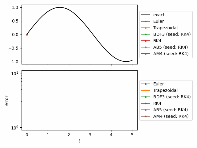
This can be done with solve_ivp but one would have to store the entire solution for each solve in memory and then loop again to perform the plotting. That doesn't sound so bad for a system with only two variables (since it's a second order equation), but this becomes immensely important when you want to solve PDEs where the number of dimensions can easily be in the thousands or millions.

Memory Efficient

For example, I used odeiter to solve a neural field equation on a bumpy-sphere. A neural field equation is an integro-differential equation, so the resulting ODE had hundreds of thousands of dimensions, one for each sample point on the surface. At each time step, I plot the solution (left) and I also plot the maximum value of the solution (right) as a continuous path across the surface.

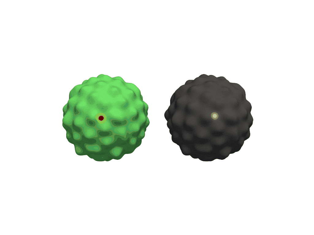
Once a frame for the animation is generated, the solution at that time point is no longer required so it is discarded and the memory is reclaimed.

Lazy

Another advantage, is that generators are lazy. They don't compute the solution until you ask for it. This allows you to run simulations without a predetermined stopping condition. For example, the following animation shows two simulations created with odeiter where the difference is in the amplitudes of the forcing functions (magenta).

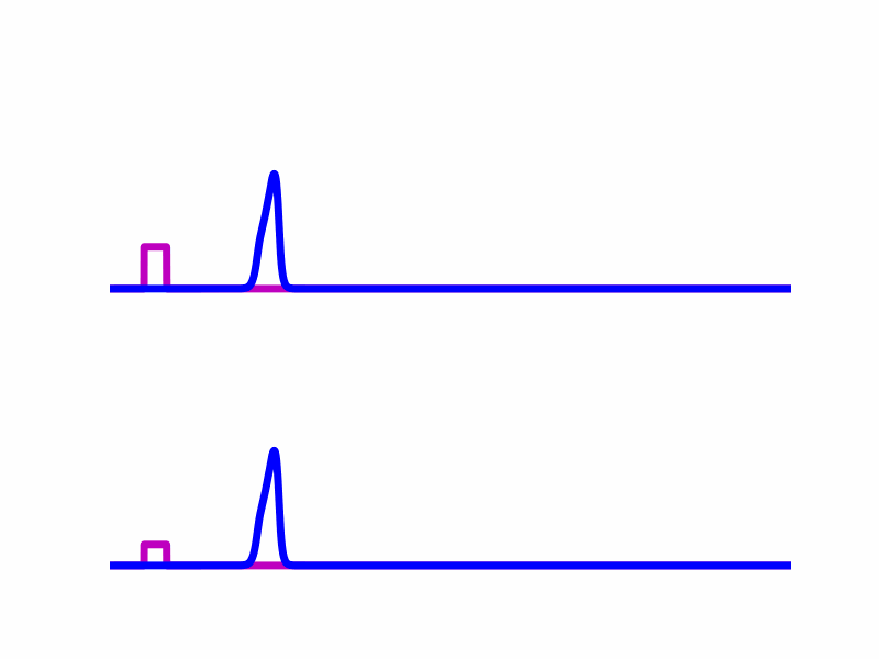
The top simulation entrains so the solution (blue) rides the forcing function (magenta) indefinitely, and achieves a stable traveling wave solution. In the bottom simulation, the solution rides the forcing function for a while but in the end it does not entrain because the forcing function is too weak. I tested many amplitudes and simulated until either they reached a traveling pulse solution or until the forcing term was separated from the solution by a certain distance. I was able to implement this easily without needing to know how long the simulation would need to run.